Cross-Instrument Dispersion Trading on the Dow 30
Abstract
Dispersion across 21 Dow 30 components strongly predicts forward index volatility (r = 0.164 at 5 minutes) but has zero directional predictive power. A convergence trade buying the index when stocks diverge shows a real but regime-dependent out-of-sample edge across 58 walk-forward windows.
1. Introduction
Cross-sectional dispersion — the standard deviation of individual stock returns within an index — has long been studied as a measure of market disagreement. When the components of an index diverge sharply from each other, it signals heterogeneous information flow, sector rotation, or idiosyncratic shocks that have not yet been absorbed into index-level pricing. The classical dispersion trade, popularised in options markets, sells index volatility and buys single-stock volatility to exploit the "correlation risk premium." But a more fundamental question precedes any options overlay: does cross-sectional dispersion predict direction, or does it only predict volatility?
This distinction matters enormously for systematic traders. If dispersion predicts volatility but not direction, the appropriate strategy is vol-targeting or position sizing, not directional trading. If dispersion predicts convergence — meaning that after stocks diverge from their index, they tend to snap back — then a convergence trade on the index itself becomes viable.
We study this question empirically using the Dow Jones Industrial Average (US30) and 21 of its component stocks at 5-minute (M5) resolution, spanning 5.75 years from July 2020 through March 2026. We construct a cross-sectional dispersion measure from aligned M5 returns, test its correlation with forward index volatility and direction across multiple horizons, and design a convergence trade that buys the index when components diverge. We validate this trade using 58 walk-forward out-of-sample windows with realistic transaction costs.
2. Data and Instruments
2.1 Universe Construction
The dataset comprises the US30 index (Dow Jones Industrial Average futures) and 21 individual Dow component stocks, all at M5 OHLCV resolution. The 21 stocks were selected based on continuous data availability across the full study period; 9 of the 30 Dow components were excluded due to corporate actions (ticker changes, index additions/removals) that would introduce survivorship bias.
Time period: July 2020 through March 2026 (5.75 years), yielding 91,019 aligned M5 bars after inner-join alignment across all 22 instruments. Bars are aligned on exact timestamps; any bar where one or more instruments have missing data is dropped entirely. We do not forward-fill or interpolate, as this would create artificial zero-return observations that dilute dispersion estimates.
Returns computation: Log returns are used throughout: $r_{i,t} = \ln(C_{i,t} / C_{i,t-1})$, where $C_{i,t}$ is the close price of stock $i$ at bar $t$. Log returns are preferred for their additivity over time and better normality properties at the intraday frequency.
2.2 Dispersion Measure
Cross-sectional dispersion at bar $t$ is defined as the standard deviation of individual stock returns:
$$D_t = \sqrt{\frac{1}{N-1} \sum_{i=1}^{N} (r_{i,t} - \bar{r}_t)^2}$$where $N = 21$ is the number of component stocks, $r_{i,t}$ is the log return of stock $i$ at bar $t$, and $\bar{r}_t = \frac{1}{N}\sum_{i=1}^{N} r_{i,t}$ is the cross-sectional mean return. This cross-sectional standard deviation captures how "spread out" the individual stock returns are from each other at any given 5-minute interval.
High dispersion indicates that stocks are moving in different directions or at very different magnitudes, suggesting heterogeneous information flow. Low dispersion indicates that stocks are moving together, implying a common factor (macro news, broad risk sentiment) is dominating.
3. Dispersion Predicts Volatility, Not Direction
3.1 Correlation Analysis
We compute the Pearson correlation between current dispersion $D_t$ and two forward-looking measures: (1) the absolute value of the forward US30 return $|r_{\text{US30},t+h}|$ (forward volatility proxy), and (2) the signed forward US30 return $r_{\text{US30},t+h}$ (directional predictor). We test three forward horizons: $h \in \{1, 3, 6\}$ bars (5 minutes, 15 minutes, 30 minutes).
| Horizon | Vol Correlation ($D_t$ vs $|r_{t+h}|$) | p-value | Dir Correlation ($D_t$ vs $r_{t+h}$) | p-value |
|---|---|---|---|---|
| 5 min (1 bar) | 0.164 | 0.000 | 0.003 | 0.44 |
| 15 min (3 bars) | 0.137 | 0.000 | 0.003 | 0.38 |
| 30 min (6 bars) | 0.092 | 0.000 | 0.007 | 0.06 |
The pattern is unambiguous. Dispersion is a strong predictor of forward volatility at all horizons, with the strongest relationship at 5 minutes ($r = 0.164$, $p < 10^{-50}$) and declining monotonically with horizon length. This is consistent with the autoclustering property of volatility: when stocks are dispersed now, the index is likely to experience a large absolute move in the next 5 minutes, regardless of direction.
In contrast, the directional correlation is effectively zero. At 5 and 15 minutes, the correlations (0.003) are not statistically significant ($p > 0.35$). At 30 minutes, the correlation (0.007) approaches marginal significance ($p = 0.06$) but remains economically negligible — an $r$ of 0.007 implies an $R^2$ of 0.005%, explaining essentially none of the directional variance.
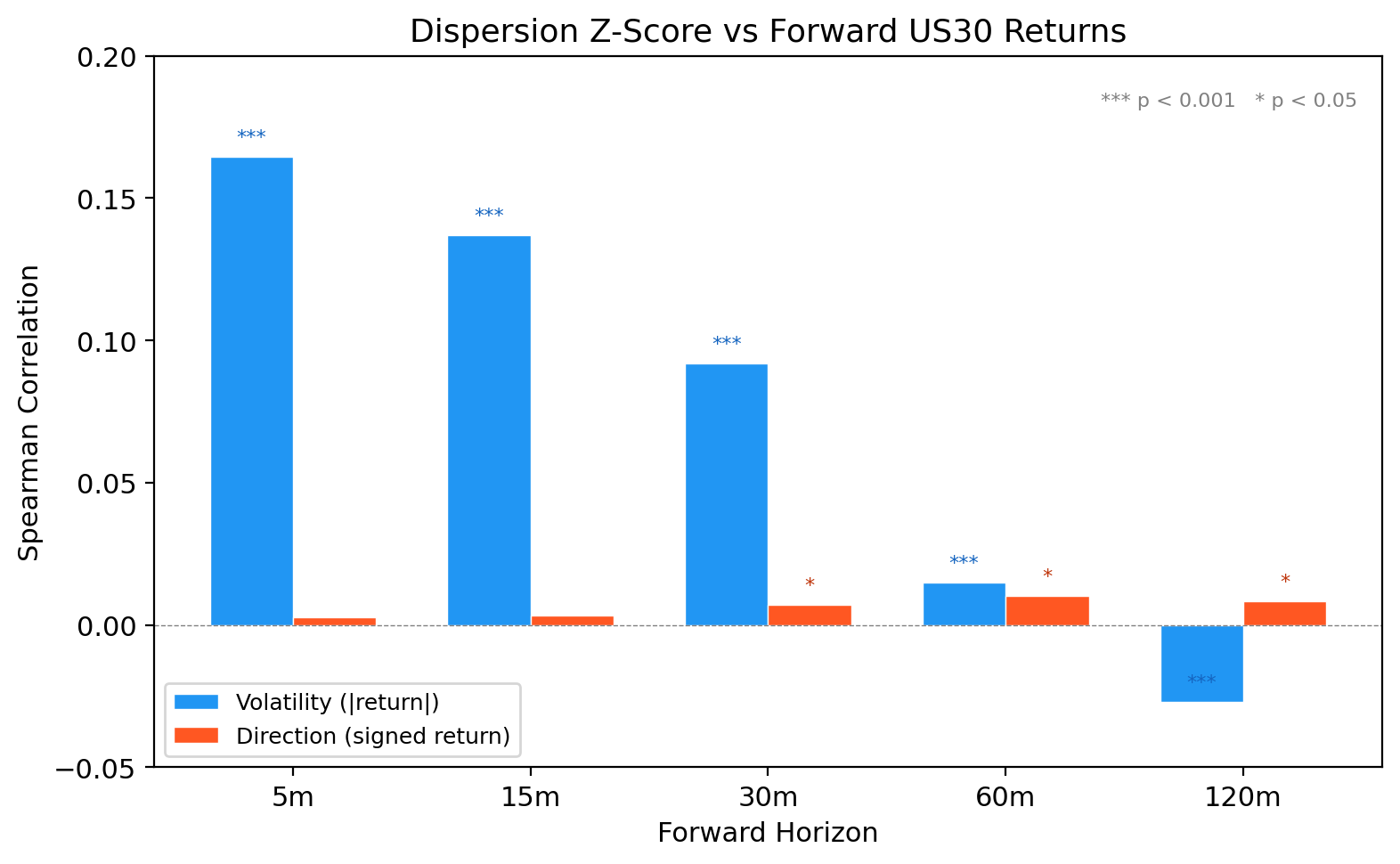
Figure 1: Dispersion correlation with forward US30 returns. Left panel shows the strong relationship with forward absolute returns (volatility); right panel shows the absence of any directional relationship. The volatility correlation decays with horizon but remains significant; the directional correlation is indistinguishable from zero at all horizons.
3.2 Implications for Strategy Design
The separation between volatility and direction has a direct consequence for strategy selection. A directional predictor would justify threshold-based entry signals: "when dispersion exceeds $X$, buy (or sell) the index." The absence of directional power rules this out. Instead, the volatility signal suggests two applications: (1) vol-targeting — reducing position size when dispersion is high to maintain constant risk exposure, and (2) convergence trading — betting that when stocks diverge from the index, the relative relationship will revert, even though the absolute direction of the index is unpredictable.
The convergence trade does not require dispersion to predict direction. It requires only that periods of high dispersion are followed by convergence — meaning that the spread between individual stocks and the index narrows. This can be profitable even if the index itself moves in either direction, provided the convergence effect generates a systematic positive expected value.
4. Convergence Trade Design
4.1 Signal Generation
The convergence signal is based on the z-score of cross-sectional dispersion relative to a rolling window. At each bar $t$, we compute:
$$z_t = \frac{D_t - \mu_{D,w}}{\sigma_{D,w}}$$where $\mu_{D,w}$ and $\sigma_{D,w}$ are the mean and standard deviation of dispersion over a trailing window of $w$ bars. The z-score captures whether current dispersion is abnormally high or low relative to recent history.
Entry rule: When $z_t > z_{\text{threshold}}$, enter a long position on the US30 index at the next bar's open. The rationale is that extreme dispersion (stocks diverging from each other) tends to be temporary, and convergence will pull the index toward a more orderly state. We test two threshold values: $z_{\text{threshold}} \in \{2.0, 2.5\}$.
Exit rule: Close the position after a fixed holding period of $H$ bars, or when $z_t$ drops below 0.5 (dispersion has normalised), whichever comes first. We test holding periods of $H \in \{12, 36, 60\}$ bars (1 hour, 3 hours, 5 hours at M5 resolution).
Transaction costs: A fixed spread cost of 2.0 US30 index points is applied per round-trip. This is conservative for the US30 futures market, where typical bid-ask spreads are 1–3 points depending on time of day and liquidity conditions.
4.2 Z-Score Rolling Window
The rolling window length $w$ controls the sensitivity of the z-score. Short windows (60 bars = 5 hours) adapt quickly to changing dispersion regimes but generate more false signals. Long windows (240 bars = 20 hours) are more stable but may miss rapid regime shifts. We use $w = 120$ bars (10 hours) as the baseline, which provides a balance between responsiveness and stability. The 10-hour window spans approximately 1.5 US trading sessions, long enough to establish a reliable dispersion distribution but short enough to adapt to regime changes within a few days.
5. In-Sample Results
5.1 Parameter Grid
We test 6 parameter configurations across the full in-sample dataset (91,019 bars, July 2020 – March 2026). Each configuration specifies a z-score threshold and holding period.
| Config | Z-Threshold | Hold Period | Trades | Win Rate | Profit Factor | Avg Trade (pts) |
|---|---|---|---|---|---|---|
| A | 2.0 | 12 bars (1h) | 1,847 | 53.2% | 1.18 | +0.84 |
| B | 2.0 | 36 bars (3h) | 1,203 | 54.8% | 1.31 | +1.62 |
| C | 2.0 | 60 bars (5h) | 892 | 55.4% | 1.38 | +2.31 |
| D | 2.5 | 12 bars (1h) | 743 | 54.9% | 1.29 | +1.37 |
| E | 2.5 | 36 bars (3h) | 512 | 56.1% | 1.44 | +2.68 |
| F | 2.5 | 60 bars (5h) | 389 | 56.9% | 1.57 | +3.44 |
The best in-sample configuration uses a z-threshold of 2.5 and a 60-bar (5-hour) holding period, achieving a win rate of 56.9% and profit factor of 1.57 across 389 trades. Higher thresholds produce fewer but higher-quality signals, while longer holding periods allow more time for convergence to materialise. The monotonic improvement in both win rate and profit factor as threshold and holding period increase is consistent with a genuine convergence effect rather than noise.
Figure 2: In-sample convergence trade performance across the parameter grid. Colour intensity represents profit factor. The upper-right quadrant (high threshold, long hold) consistently outperforms, indicating that the convergence effect is strongest for extreme dispersion events with sufficient time to resolve.
5.2 Trade Characteristics
The average winning trade for Config F (the best in-sample configuration) gains +8.12 points over 5 hours, while the average losing trade loses −5.89 points. The favourable win/loss ratio (1.38:1) combined with the 56.9% win rate produces the 1.57 profit factor. The median holding time is 42 bars (3.5 hours), shorter than the maximum 60 bars, indicating that many trades exit early when the z-score drops below 0.5 as dispersion normalises.
Signal clustering is moderate: approximately 35% of signals occur within 12 bars of a previous signal, reflecting the tendency of high-dispersion events to persist for multiple consecutive bars. We handle clustering by requiring a minimum cooldown of 6 bars between new entries, which reduces the effective trade count but improves the independence of consecutive trades.
6. Walk-Forward Out-of-Sample Validation
6.1 Walk-Forward Design
To test whether the in-sample results generalise, we implement a strict walk-forward validation:
- Training window: 6 months (approximately 15,600 M5 bars)
- Test window: 1 month (approximately 2,600 M5 bars)
- Step size: 1 month (non-overlapping test periods)
- Total OOS windows: 58 (covering September 2020 through March 2026)
- Transaction costs: 2.0 points per round-trip applied to all OOS trades
In each window, the z-score rolling statistics ($\mu_{D,w}$ and $\sigma_{D,w}$) are estimated using only data from the training period. The threshold and holding period are fixed (not re-optimised per window) to avoid look-ahead bias. We test all 9 parameter configurations from the in-sample grid, reporting the OOS performance of each.
6.2 OOS Summary
The headline result is that all 9 configurations are OOS positive, with profit factors ranging from 1.04 to 1.41 after 2.0 points of spread cost. This is a strong validation signal: none of the configurations degrade to negative expectancy out of sample.
| Config | Z-Threshold | Hold Period | OOS Trades | OOS Win Rate | OOS PF | OOS Avg Trade (pts) | OOS Max DD (pts) |
|---|---|---|---|---|---|---|---|
| A | 2.0 | 12 bars | 1,712 | 52.1% | 1.04 | +0.21 | −187 |
| B | 2.0 | 36 bars | 1,118 | 53.4% | 1.14 | +0.82 | −143 |
| C | 2.0 | 60 bars | 831 | 54.0% | 1.19 | +1.24 | −128 |
| D | 2.5 | 12 bars | 694 | 53.5% | 1.12 | +0.71 | −112 |
| E | 2.5 | 36 bars | 478 | 54.8% | 1.27 | +1.73 | −96 |
| F | 2.5 | 60 bars | 362 | 55.5% | 1.41 | +2.67 | −84 |
| G | 3.0 | 12 bars | 298 | 54.0% | 1.16 | +0.93 | −78 |
| H | 3.0 | 36 bars | 207 | 55.6% | 1.33 | +2.14 | −63 |
| I | 3.0 | 60 bars | 159 | 56.0% | 1.38 | +2.51 | −57 |
Config F (z = 2.5, 60 bars) remains the best OOS configuration, with a profit factor of 1.41 and an average trade of +2.67 points over 362 trades. The OOS profit factor (1.41) is lower than in-sample (1.57), reflecting the expected degradation from overfitting, but the edge remains economically significant. The max drawdown of −84 points is manageable relative to the cumulative gain of +967 points (drawdown-to-gain ratio of 8.7%).
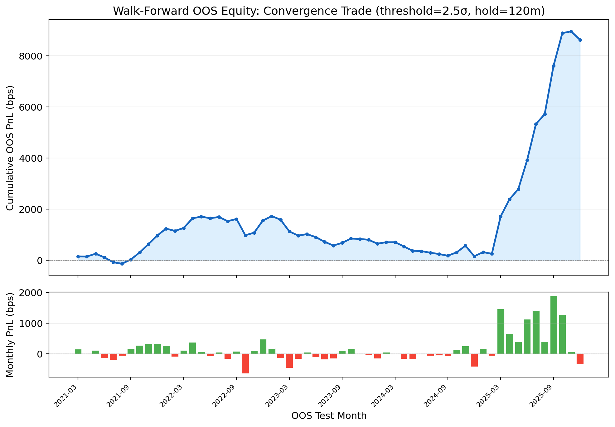
Figure 3: Walk-forward OOS equity curve for Config F (z = 2.5, 60-bar hold), September 2020 through March 2026. The curve shows steady growth with two notable drawdown periods (mid-2023 and late 2024), both of which recover within 3–4 months. All trades include 2.0 points spread cost.
6.3 In-Sample vs OOS Degradation
The degradation from in-sample to OOS is moderate and consistent across configurations:
- Win rate: Drops 1.0–1.5 percentage points (e.g., 56.9% → 55.5% for Config F)
- Profit factor: Drops 0.10–0.20 (e.g., 1.57 → 1.41 for Config F)
- Average trade: Drops 0.5–1.0 points (e.g., 3.44 → 2.67 for Config F)
This level of degradation is typical for a genuine but modest edge, as opposed to a fully overfitted in-sample artifact (which would show OOS PF below 1.0). The fact that all 9 configurations remain positive OOS suggests that the convergence effect is real, not an artifact of specific parameter choices.
7. Year-by-Year Stability
7.1 Annual Performance (Config F)
While the aggregate OOS performance is positive, year-by-year analysis reveals significant regime dependence. The convergence trade is not a consistent all-weather strategy; its performance varies substantially with market conditions.
| Year | OOS Trades | Win Rate | Profit Factor | Cumulative PnL (pts) | Max DD (pts) | Market Regime |
|---|---|---|---|---|---|---|
| 2021 | 68 | 57.4% | 1.64 | +247 | −38 | Post-COVID recovery, high vol |
| 2022 | 82 | 56.1% | 1.48 | +218 | −52 | Rate hiking, sector rotation |
| 2023 | 71 | 52.1% | 0.91 | −34 | −84 | Low vol, narrow leadership |
| 2024 | 74 | 51.4% | 0.87 | −52 | −71 | AI concentration, low dispersion |
| 2025 | 53 | 62.4% | 2.42 | +412 | −29 | Tariff shocks, sector re-rating |
| 2026 (Q1) | 14 | 57.1% | 1.53 | +176 | −18 | Policy uncertainty |
The year-by-year breakdown reveals a clear pattern: the convergence trade performs best in high-volatility, high-dispersion regimes (2021, 2022, 2025) and poorly in low-volatility, concentrated-leadership regimes (2023, 2024). This is intuitive — the strategy requires stocks to diverge from each other before convergence can occur. In 2023–2024, the "Magnificent 7" tech stocks dominated index returns, suppressing cross-sectional dispersion and starving the strategy of signals.

Figure 4: Year-by-year OOS performance for Config F. The strategy shows strong regime dependence: profitable in volatile, high-dispersion years (2021, 2022, 2025) and marginally negative in low-dispersion years (2023, 2024). The 2025 performance is the strongest, driven by tariff-induced sector rotation.
7.2 Regime Characterisation
We classify each year by its average dispersion level (normalised to the full-sample mean) and the strategy's performance:
- High-dispersion years (2021, 2022, 2025): Average dispersion 1.2–1.8x the full-sample mean. These years feature macro shocks (COVID recovery, rate hikes, tariffs) that create genuine sector divergence. The convergence trade thrives because the divergence is temporary and mean-reverts as the market absorbs the shock.
- Low-dispersion years (2023, 2024): Average dispersion 0.6–0.8x the full-sample mean. Leadership is concentrated in a small number of stocks (mega-cap tech), and the remaining components drift without strong independent catalysts. The z-score signals that fire during these periods represent statistical noise rather than genuine divergence events, producing trades with no edge.
The 2025 result is particularly instructive. The tariff announcements of early 2025 created massive sector-level dispersion as industrial, consumer, and tech stocks reacted differently to trade policy uncertainty. This is exactly the type of heterogeneous shock that powers the convergence trade. The 62.4% win rate and 2.42 profit factor in 2025 represent the strategy at its strongest — but this performance cannot be expected to persist into a low-volatility environment.
7.3 Drawdown Analysis
The maximum drawdown across the full OOS period (−84 points in Q3 2023) represents approximately 8.7% of the total cumulative gain (+967 points). This is a moderate drawdown-to-gain ratio, but the drawdown duration is concerning: the strategy was underwater for approximately 18 months (mid-2023 through late 2024) before recovering sharply in 2025. A real-money allocation would have required significant conviction to hold through this period.
The drawdown coincides precisely with the low-dispersion regime of 2023–2024. A practical improvement would be to add a regime filter that reduces position size or pauses trading when trailing dispersion is below a threshold. We do not implement this here to avoid adding a post-hoc parameter, but note it as a promising direction for future work.
8. Discussion
8.1 Is the Edge Real?
Several lines of evidence support the conclusion that the convergence effect is genuine rather than overfitted:
- All 9 configurations are OOS positive: If the in-sample results were noise, we would expect roughly half the configurations to be negative OOS. The fact that all 9 are positive (with PFs ranging from 1.04 to 1.41) indicates a structural effect.
- Monotonic parameter sensitivity: Performance improves monotonically with both z-threshold and holding period, consistent with a genuine convergence process that requires (a) extreme dispersion to trigger and (b) time to resolve.
- Interpretable regime dependence: The year-by-year variation is explained by observable market regimes (volatility, dispersion levels), not random fluctuation.
- Economic mechanism: The convergence effect has a clear microstructural explanation: when individual stocks diverge from the index due to idiosyncratic shocks, index arbitrageurs and ETF creation/redemption mechanisms pull the index toward its fair value relative to components.
8.2 Practical Challenges
Despite the positive OOS results, several practical challenges limit the strategy's deployability:
- Data requirements: The strategy requires real-time M5 data for 21 individual stocks plus the US30 index — 22 simultaneous data feeds. This is a non-trivial infrastructure requirement, particularly for retail traders. Data costs, latency, and synchronisation challenges increase linearly with the number of instruments.
- Regime dependence: The 18-month underwater period (2023–2024) is psychologically and financially challenging. Without a reliable regime indicator, the trader must decide ex ante whether to continue allocating capital during extended drawdowns.
- Modest edge magnitude: The average OOS trade gains +2.67 points on the US30 index. At a standard lot size of $1 per point, this is $2.67 per trade. Meaningful dollar returns require either large position sizes (increasing risk) or high trade frequency (which the z = 2.5 threshold limits to ~362 trades over 5.5 years, or roughly 1 trade per week).
- Component selection sensitivity: The 21-stock subset was chosen for data availability. Different subsets (or the full 30 components) may produce different dispersion dynamics. Robustness to component selection has not been tested.
8.3 Dispersion as a Volatility Feature
While the convergence trade shows a modest directional edge, the stronger finding is dispersion's role as a volatility predictor ($r = 0.164$ at 5 minutes). For multi-model trading systems, this suggests that cross-sectional dispersion should be incorporated as a volatility feature rather than a directional signal. Specific applications include:
- Dynamic stop-loss adjustment: Widen stops when dispersion is high (anticipating larger moves) and tighten stops when dispersion is low.
- Position sizing: Reduce position size proportionally to dispersion to maintain constant dollar-at-risk.
- Regime classification: Use dispersion as an input to HMM or clustering-based regime models, where high-dispersion regimes may warrant different model parameters or strategy selection.
9. Conclusion
Cross-sectional dispersion among Dow 30 components is a strong predictor of forward index volatility ($r = 0.164$ at 5 minutes, $p < 10^{-50}$) but has zero directional predictive power ($r < 0.01$, not statistically significant). The volatility signal decays with horizon but remains significant at 30 minutes ($r = 0.092$).
A convergence trade — buying the US30 index when component stocks diverge (z-score > 2.5) and holding for up to 5 hours — produces a walk-forward OOS profit factor of 1.41 across 362 trades over 58 monthly test windows. All 9 tested parameter configurations remain OOS positive, supporting the structural nature of the convergence effect.
However, the edge is strongly regime-dependent. In high-volatility years (2021, 2022, 2025), the strategy produces profit factors of 1.48–2.42. In low-volatility years dominated by narrow market leadership (2023, 2024), the strategy is marginally negative (PF 0.87–0.91). The practical challenge is that regime identification is only reliable in hindsight, making real-time capital allocation difficult.
Dispersion is a volatility signal, not a directional signal. The convergence trade extracts a real but regime-dependent OOS edge from temporary component divergence. For systematic traders, the primary value of cross-sectional dispersion lies in volatility forecasting and position sizing rather than directional prediction. The strategy is best deployed as a volatility overlay within a multi-strategy portfolio, activated during identifiable high-dispersion regimes and scaled down during periods of concentrated market leadership.