Transformer Models vs SSMs for Financial Time Series
Abstract
We present GoldSSM, a selective state space model for intraday gold price direction forecasting. The architecture combines a Variable Selection Network, a stack of Mamba blocks with selective scan, and temporal attention pooling. At 2.0M parameters, GoldSSM serves as a drop-in replacement for Transformer-based models with identical forward signatures, while offering linear-time sequence processing and improved handling of long-range dependencies in financial time series.
1. Introduction
Intraday price forecasting in liquid financial markets (commodities, FX, equity indices) is driven by monetary policy expectations, real interest rate movements, currency dynamics, cross-asset risk appetite, and market microstructure such as liquidity sweeps, order flow imbalances, and session transitions. These drivers interact nonlinearly, and their relative importance is time-varying and regime-dependent. We develop GoldSSM using XAUUSD (gold) as our primary instrument, chosen for its high liquidity ($130B+ daily turnover), diverse driver set, and strong regime structure. The architecture generalises to any liquid financial instrument at the intraday timescale.
Three challenges define intraday forecasting at the one-minute (M1) timescale:
- Extremely low signal-to-noise ratio. At M1 resolution, most price bars contain no directional information. Signal concentrates in a sparse subset of bars: those coinciding with macroeconomic releases, liquidity sweeps near key levels, and session-boundary transitions. A model that treats all timesteps uniformly will be overwhelmed by noise.
- Non-stationarity at every timescale. The statistical properties of financial returns, including volatility, autocorrelation structure, cross-asset correlations, and individual feature relevance, shift continuously. A volatility regime that persists for weeks can collapse within minutes during a macro shock. Models with frozen normalisation statistics or static feature weights degrade as the market evolves.
- No fixed optimal lookback horizon. How much historical context an accurate forecast requires depends on the current regime. Trend-following signals need long lookback windows (hours to half-days); mean-reversion signals around support/resistance levels need short, precise context (tens of minutes). A model locked to one temporal scale will systematically underperform whenever a different scale dominates.
Existing deep learning approaches do not address these challenges simultaneously. LSTMs (Hochreiter and Schmidhuber, 1997) process sequences through a single fixed lookback window with uniform temporal aggregation and offer no mechanism to attend selectively to informative bars or adapt feature weighting across regimes. Transformers (Vaswani et al., 2017) introduce flexible attention over the full sequence, but at $O(T^2 \cdot d)$ cost, making context windows beyond 200 bars impractical for real-time M1 inference. Efficient variants such as Informer (Zhou et al., 2021) reduce the quadratic bottleneck but retain static feature treatment and fixed positional encodings. In all these architectures, feature selection is performed offline (e.g., via AUC screening or LASSO) and remains frozen during inference, even though feature relevance rotates with market regime.
This paper introduces GoldSSM, a structured state space architecture that addresses all three limitations. GoldSSM combines a Variable Selection Network for dynamic, regime-aware feature weighting; multi-scale Mamba encoding with input-dependent state transitions for linear-time sequence processing; learned temporal attention pooling to concentrate summary capacity on informative bars; and adaptive stream gating to redistribute emphasis across temporal scales as the regime shifts. GoldSSM processes 12 hours of M1 context (720 bars) in linear time, with approximately 2.1× fewer parameters than the equivalent Transformer baseline.
2. The Transformer Problem for Financial Time Series
Why do Transformer models, despite their dominance in natural language processing, perform poorly on intraday financial time series? The limitations go beyond computation. They reflect structural mismatches between the assumptions embedded in self-attention and the statistical properties of financial data.
2.1 Quadratic Complexity
The core operation of a Transformer encoder is scaled dot-product self-attention:
$$\text{Attention}(Q, K, V) = \text{softmax}\left(\frac{QK^\top}{\sqrt{d_k}}\right)V$$where $Q, K, V \in \mathbb{R}^{T \times d}$. The $QK^\top$ matrix multiplication alone requires $O(T^2 \cdot d)$ operations, and the resulting $T \times T$ attention matrix must be materialised in memory. For a 720-bar M1 window (12 hours of trading), this produces 518,400 attention score pairs per head per layer. With multiple heads and layers, the total computational burden makes real-time inference on commodity GPU hardware infeasible. This cost applies to each temporal context window the model must process.
Quadratic scaling forces a trade-off between context richness and computational tractability. Practitioners must either truncate the context window, discarding potentially valuable regime information from earlier in the session, or accept latency that exceeds the bar interval. Neither option is acceptable for a production system where inference must complete within the bar boundary.
2.2 Uniform Attention over Noise
Self-attention treats every timestep as potentially relevant to every other. For natural language this is sensible: any word in a sentence may modify the meaning of any other. For financial time series it is unsuitable. At M1 resolution, over 95% of bars contain no actionable directional information. Signal concentrates in a sparse, irregular subset of timesteps: bars coinciding with macroeconomic data releases (NFP, CPI, FOMC), liquidity sweeps past key support/resistance levels, and session-boundary transitions (London open, New York open).
In principle, the softmax attention mechanism can assign near-zero weight to uninformative bars. In practice, the learning problem is severely complicated by the low signal-to-noise ratio. The model must discover which bars are informative from data where such bars are rare events and where "informative" itself changes across regimes. Attention maps end up spreading probability mass diffusely across the sequence, diluting the signal from the few bars that matter.
2.3 Static Feature Weighting
Transformers process a fixed feature vector at each timestep with no native mechanism to adapt which features receive emphasis based on market state. In financial markets, feature relevance rotates: momentum and moving-average distance dominate trending regimes; support/resistance proximity and volatility dominate mean-reverting regimes; cross-asset correlations and rate-sensitivity features become paramount during macro shocks. A Transformer treats the input vector identically regardless of regime, relying on general model capacity to implicitly learn regime-dependent feature interactions. Given the non-stationarity of financial data, this implicit approach is data-inefficient and prone to overfitting.
2.4 Positional Encoding Assumes Regularity
Standard Transformer positional encodings, whether sinusoidal or learned, assume that information density is roughly uniform across sequence positions. Financial time series violate this assumption. An overnight gap compresses hours of calendar time into a single bar transition. A session open concentrates information that accumulated during the preceding close into the first few bars. A macro release injects an information spike that decays over subsequent bars. The regular positional grid has no way to represent this irregular density, and the model wastes capacity learning to ignore the positional signal during periods where it misleads.
3. The State Space Alternative
State space models (SSMs) take a different approach to sequence modelling. Instead of computing pairwise interactions between all timesteps, an SSM maintains a compressed latent state vector $h_t$ that is updated recurrently as each new observation arrives. Computational complexity is $O(T)$ in sequence length, making long context windows practical without architectural compromise.
3.1 Classical State Space Formulation
A continuous-time state space model defines the relationship between input $u(t)$ and output $y(t)$ through a latent state $h(t) \in \mathbb{R}^N$:
$$h'(t) = A \, h(t) + B \, u(t), \qquad y(t) = C \, h(t) + D \, u(t)$$where $A \in \mathbb{R}^{N \times N}$ governs the state dynamics, $B \in \mathbb{R}^{N \times 1}$ controls how input enters the state, $C \in \mathbb{R}^{1 \times N}$ maps the state to output, and $D \in \mathbb{R}$ is a skip connection. The state dimension $N$ is a design hyperparameter controlling the model's memory capacity.
Classical SSMs (e.g., S4, Gu et al., 2022) use fixed, data-independent parameters $A$, $B$, and $C$. This allows efficient computation via convolutional or recurrent modes but imposes a limitation: memory dynamics are identical regardless of input content. A noise-dominated consolidation bar and a macro-shock bar receive the same state update treatment.
3.2 Mamba: Input-Dependent State Transitions
The Mamba architecture (Gu and Dao, 2023) introduces the key innovation that makes SSMs viable for financial time series: input-dependent state transition parameters. Rather than using fixed $B$, $C$, and discretisation step $\Delta$, Mamba computes these from the current input:
$$\Delta_t = \text{softplus}(W_\Delta \, u_t), \quad B_t = W_B \, u_t, \quad C_t = W_C \, u_t$$The discretisation step $\Delta_t$ controls the effective memory horizon at each timestep. A large $\Delta_t$ causes the state to incorporate the current input strongly while decaying past information; a small $\Delta_t$ preserves the existing state with minimal update. This is computed via Zero-Order-Hold (ZOH) discretisation:
$$\bar{A}_t = \exp(\Delta_t \odot A), \quad \bar{B}_t = \Delta_t \odot B_t \odot u_t$$The discrete-time state update and output equations are then:
$$h_t = \bar{A}_t \odot h_{t-1} + \bar{B}_t, \quad y_t = C_t^\top h_t + D \odot u_t$$In financial terms, each bar chooses how much historical context to retain based on its own content. During a persistent trend or volatility regime, the model can learn small $\Delta_t$ values, allowing macro-shock information to persist in the state over hundreds of bars. During noisy, low-information periods, large $\Delta_t$ values cause rapid state decay, discarding stale context within a few steps. This adaptive memory horizon, learned end-to-end from data, is well suited to a market where the optimal lookback window shifts continuously.
3.3 Computational Advantage
Per-step complexity of a Mamba block is $O(d \cdot N)$, where $d$ is the embedding dimension and $N$ is the state dimension. Over a sequence of length $T$, total complexity is $O(T \cdot d \cdot N)$. With $d = 128$ and $N = 8$, a 720-bar window requires approximately 737,280 multiply-accumulate operations, compared to 518,400 attention score pairs per head for a single Transformer layer before accounting for value projection and multi-head aggregation.
The SSM computation is causal by construction: $h_t$ depends only on $h_{t-1}$ and $u_t$. No future information can leak into the prediction, and no explicit positional encoding is needed because the causal state update inherently encodes temporal position through accumulated state dynamics. Both properties suit financial time series, where causality is a hard constraint and information density is irregular.
4. GoldSSM Architecture
GoldSSM is a multi-scale state space architecture for intraday financial time series forecasting. Rather than processing a single fixed-length context window, it processes multiple parallel temporal streams at different horizons. Our implementation uses four streams (60, 120, 240, and 720 M1 bars, spanning 1 to 12 hours), though the number and length of streams are configurable. The architecture has four components arranged in a pipeline, each addressing a limitation identified in Section 2.
4.1 Variable Selection Network
The first stage is a Variable Selection Network (VSN), inspired by the gating mechanism in Temporal Fusion Transformers (Lim et al., 2021) but adapted for financial feature selection. The VSN learns a weight vector over the input feature space at every bar, conditioned on the current observation and a global regime context vector:
$$w_t = \text{softmax}\big(\text{MLP}([x_t \; ; \; c])\big) \in \mathbb{R}^F$$where $x_t \in \mathbb{R}^F$ is the raw feature vector at bar $t$, $c$ is a learned regime context embedding, and $[\; ; \;]$ denotes concatenation. The softmax normalisation ensures the weights form a valid probability distribution over features, giving interpretable feature importance at every bar.
The selected features are then processed through two complementary pathways:
- Value path: $v_t = W_v(x_t \odot w_t)$ carries the current numeric signal, element-wise gated by the selection weights. Features irrelevant to the current regime are multiplicatively suppressed before entering the encoder.
- Prototype path: $p_t = w_t^\top P$ carries a learned feature identity prior, where $P \in \mathbb{R}^{F \times d}$ is a learnable prototype matrix. This path encodes which features are active regardless of their numeric values, providing the encoder with a regime fingerprint.
- Regime context: $r_t = W_c \cdot c$ is a linear projection of the regime embedding that biases the combined representation toward regime-specific interpretation.
The three paths are summed to produce the VSN output: $z_t = v_t + p_t + r_t$. This design gives the model dynamic feature selection, e.g. upweighting momentum features during trends and volatility features during mean-reversion, without the memory cost of materialising an $F \times F$ feature interaction matrix. Total complexity is $O(B \times T \times \max(F, d))$, where $B$ is batch size, $T$ is sequence length, $F$ is feature count, and $d$ is embedding dimension. No outer-product or pairwise feature computation is required.
Unlike the static feature treatment of Transformers (Section 2.3), the VSN re-weights the feature space at every bar conditioned on regime context. The selection weights $w_t$ also serve as a diagnostic: they reveal which features the model considers most informative at any given moment, an interpretability benefit absent from standard Transformer encoders.
4.2 Multi-Scale Mamba Encoding
Encoded features from the VSN feed into four parallel Mamba streams at different temporal scales: 60 bars (1 hour), 120 bars (2 hours), 240 bars (4 hours), and 720 bars (12 hours). Each stream has an identical architecture:
- Variable Selection: A dedicated VSN instance (Section 4.1) produces regime-aware feature representations for the stream's temporal window.
- Mamba blocks (2 layers): Each Mamba block consists of a depth-wise causal convolution (kernel size 4) followed by the selective state space scan. The causal convolution captures local patterns such as candlestick formations and short-term momentum; the SSM then integrates them into the long-range latent state. The scan applies the input-dependent state update equations from Section 3.2 across the full sequence in linear time.
- Output gating: The Mamba block output passes through a SiLU-gated linear projection: $\text{out}_t = \text{SiLU}(W_g \, h_t) \odot (W_o \, h_t)$. This non-linear modulation allows the block to suppress uninformative timesteps before passing to the next stage.
- Temporal Attention Pooling: The pooling mechanism described in Section 4.3 summarises the encoded sequence into a fixed-dimensional representation.
Per-stream complexity is $O(T \cdot d \cdot N)$, where $T$ is the stream's sequence length, $d = 128$ is the embedding dimension, and $N = 8$ is the state dimension. For the longest stream (720 bars), this amounts to roughly 737,280 multiply-accumulate operations per Mamba block, a fraction of what a single Transformer attention layer costs over the same sequence length. Linear-time scaling is the reason GoldSSM can process a 720-bar (12-hour) context window directly rather than truncating history to keep quadratic attention costs within budget.
The multi-scale design addresses the variable lookback problem from Section 1. Rather than committing to a single temporal resolution, GoldSSM maintains four parallel views of the market. The 60-bar stream captures short-term microstructure and level-proximity dynamics; the 120-bar stream spans typical mean-reversion cycles; the 240-bar stream covers half-session trend structures; and the 720-bar stream provides full-session context including overnight developments and macro-regime persistence. Stream gating (Section 4.4) learns to weight these views adaptively based on the current regime.
4.3 Temporal Attention Pooling
After Mamba encoding, each stream contains a sequence of encoded representations $H = [h_1, h_2, \ldots, h_T] \in \mathbb{R}^{T \times d}$. These must be summarised into a single fixed-dimensional vector for downstream fusion and prediction. Standard approaches are inadequate here. Mean pooling dilutes signal from the few informative bars across the entire sequence. Last-token pooling discards everything except the most recent bar, forfeiting the long-range context that justified the extended window.
GoldSSM uses Temporal Attention Pooling with $Q = 4$ learned query vectors. Each query attends over the full encoded sequence via multi-head attention:
$$o_i = \text{MHA}(q_i, H, H), \quad i = 1, \ldots, Q$$ $$h_{\text{pool}} = \text{LayerNorm}\left(\frac{1}{Q}\sum_{i=1}^{Q} o_i\right)$$where $q_i \in \mathbb{R}^d$ are learnable query parameters and MHA denotes standard multi-head attention. The four queries specialise during training to attend to different aspects of the encoded sequence. In practice, certain queries attend preferentially to bars near session boundaries, others to high-volatility bars, and others to bars coinciding with cross-asset correlation shifts.
In effect, the network spends most of its summary capacity on the few bars that carry directional information instead of averaging uniformly across a sequence that is 95% noise. Computational cost is modest: $O(Q \cdot T \cdot d)$ for $Q = 4$ queries, negligible relative to the encoding stage.
This use of attention differs from Transformer self-attention in a key respect. The number of queries $Q$ is fixed and small (4), so attention computation is $O(T)$ in sequence length, not $O(T^2)$. The queries attend to the sequence; the sequence does not attend to itself.
4.4 Stream Gating and Fusion
The four pooled stream representations must be combined into a single vector for the prediction heads. Simply concatenating or averaging with equal weight ignores the fact that the most predictive temporal scale rotates across regimes: short scales dominate during mean-reversion around support/resistance levels, while long scales dominate during persistent macro-driven trends.
GoldSSM uses a Stream Gating Network that computes adaptive weights over the four streams:
$$g = 4 \cdot \text{softmax}\big(\text{MLP}(r)\big) \in \mathbb{R}^4, \quad \text{where } \sum_{i=1}^{4} g_i = 4$$where $r$ is a regime representation derived from the concatenated stream outputs. Scaling by 4 ensures an expected gate value of 1.0 per stream, preserving gradient magnitude. The gating MLP is initialised with zero weights so that all gates start at exactly 1.0 (equal weighting) and deviate only as training evidence warrants. This prevents the gating network from prematurely suppressing streams before the encoders have learned useful representations.
Gated stream representations are concatenated and projected to the prediction space:
$$z = \text{LayerNorm}\big(\text{SiLU}(W_f [g_1 \cdot h_1 \; ; \; g_2 \cdot h_2 \; ; \; g_3 \cdot h_3 \; ; \; g_4 \cdot h_4])\big)$$where $W_f$ is a linear projection and $[\; ; \;]$ denotes concatenation. The fused representation $z$ feeds three prediction heads: trade probability (sigmoid), directional probability (softmax over up/down/hold), and a reconstruction head for the auxiliary loss described in Section 6.
5. Complexity Comparison
Table 1 summarises the architectural differences between a standard Transformer encoder and GoldSSM.
| Aspect | Transformer | GoldSSM |
|---|---|---|
| Sequence complexity | $O(T^2 \cdot d)$ | $O(T \cdot d \cdot N)$ |
| At $T = 720$ (12h context) | 518,400 attention pairs per head | $720 \times 128 \times 8 = 737\text{K}$ mult-adds |
| Feature selection | Static (offline AUC screening) | Dynamic (per-timestep, regime-conditioned) |
| Temporal pooling | Mean or last-token | Learned attention (4 queries) |
| Positional encoding | Required (sinusoidal or learned) | Not needed (causal state encodes position) |
| Stream weighting | Fixed equal-weight | Regime-adaptive gating |
| Parameters | ~2.41M | ~1.15M (2.1× reduction) |
Where does the 2.1× parameter reduction come from? The Transformer baseline requires separate learned positional encodings, multi-head self-attention projections ($W_Q$, $W_K$, $W_V$, $W_O$ per head per layer), and feed-forward networks at each layer. GoldSSM replaces all of these with compact Mamba blocks whose parameter count scales as $O(d \cdot N)$ per block; the state dimension $N = 8$ is far smaller than the typical Transformer hidden dimension. The Variable Selection Network adds $O(F \cdot d)$ parameters, and the stream gating network is a small MLP. The result is approximately 1.15 million parameters at $d = 128$ (reducing to 39,634 parameters in the production deployment at $d = 16$), small enough to train on limited financial datasets without severe overfitting and fast enough for real-time M1 inference on commodity hardware.
The parameter reduction matters beyond computation. In financial machine learning, training data is inherently limited: markets have finite history, regime changes segment the data into short stationary windows, and data augmentation is problematic because synthetic financial data rarely preserves the distributional properties that matter for trading. Fewer parameters means fewer samples needed for comparable generalisation, reducing the risk of overfitting to historical idiosyncrasies that will not recur out of sample.
5.1 A Note on Practical Timing
The theoretical complexity advantage of SSMs over Transformers does not translate straightforwardly into wall-clock speedups at practical sequence lengths. Empirical timing of forward passes on GPU (CUDA) reveals that at $T = 720$, a standard Transformer encoder completes a forward pass in approximately 23ms, while GoldSSM requires approximately 411ms. The fitted scaling exponents are $T^{0.87}$ for GoldSSM and $T^{1.00}$ for the Transformer, both effectively linear at the sequence lengths tested.
The explanation lies in implementation maturity. PyTorch's self-attention benefits from years of hardware-level optimisation: FlashAttention, cuDNN-fused kernels, and memory-efficient attention backends that exploit GPU tensor cores. These optimisations compress the theoretical $O(T^2)$ scaling into near-linear observed behaviour for $T \leq 1440$. The Mamba selective scan, by contrast, relies on a sequential JIT-compiled loop that cannot yet exploit the same degree of hardware parallelism.
This does not invalidate the architectural argument. The $O(T)$ theoretical bound ensures that GoldSSM's advantage widens at longer sequence lengths where the Transformer's quadratic term eventually dominates. At $T = 10{,}000$ or beyond, the scaling difference becomes material. For the sequence lengths used in this work ($T \leq 720$), the Transformer's practical speed advantage is real and should be acknowledged. The architectural benefits of GoldSSM — in particular dynamic feature selection, adaptive memory, and regime-conditioned stream gating — remain independent of the timing comparison.
6. Training: Noise-Consistency Regularisation
Most M1 bars are noise. A model that memorises bar-level patterns will fail out of sample. The training procedure is built around this fact. The loss function combines three components:
- Direction loss (BCE): Binary cross-entropy on the predicted directional probabilities (up vs. down), providing the primary supervised signal for trade direction.
- Hold loss: A separate loss term for the trade/no-trade decision, encouraging the model to abstain from trading during ambiguous periods rather than forcing a directional prediction on every bar.
- Reconstruction loss: An auxiliary task requiring the model to reconstruct a subset of input features from the encoded representation. This regularises the encoder by ensuring it preserves general market state information, not only the features most correlated with the immediate prediction target.
The key addition is noise-consistency regularisation. During training, each input sample is processed twice: once with the original features and once with small Gaussian perturbations added. The regularisation term penalises the $L_2$ distance between the model's output logits on clean and perturbed inputs:
$$\mathcal{L}_{\text{NC}} = \mathbb{E}\left[\|f(x) - f(x + \epsilon)\|_2^2\right], \quad \epsilon \sim \mathcal{N}(0, \sigma^2 I)$$This penalty discourages the model from developing sharp decision boundaries sensitive to small input variations, which is the hallmark of overfitting to bar-level noise. A model that memorises specific bar patterns will produce dramatically different outputs when those patterns are slightly perturbed. A model that has learned genuine regime-level structure will be robust, since the regime signal spans many bars and cannot be eliminated by perturbing any single one.
6.1 Causal Normalisation
Feature normalisation is a deceptively important detail for financial time series models. Standard batch normalisation computes statistics over the entire training batch, which in a financial context means future information leaks into the normalisation of past observations. Even layer normalisation, which normalises per-sample, uses statistics from the full sequence including future timesteps.
GoldSSM uses a causal normalisation scheme with two treatment paths:
- Regime-sensitive features (36 features): Features whose distributions shift across regimes, including volatility estimates, cross-asset correlations, and momentum indicators, are normalised using a rolling 30-day z-score computed causally (using only past data at each bar). "High volatility" then means high relative to the recent past, not high relative to a global training mean that may be months stale.
- Stationary features: Features with approximately time-invariant distributions, such as time-of-day encodings, session indicators, and certain microstructure ratios, receive static z-score normalisation using training-set statistics. Rolling normalisation would not help these features and would only introduce unnecessary noise.
Assignment to one path or the other is determined empirically by measuring stationarity of each feature's rolling distribution over the training period. Features whose 30-day rolling mean or variance drifts by more than one standard deviation go to the regime-sensitive path; the rest use the stationary path.
7. Empirical Validation
To verify the claims made in this paper, we conducted a series of empirical tests on the trained GoldSSM model using the production checkpoint. The results confirm several architectural claims while revealing important caveats about computational performance.
7.1 Parameter Count
At the paper configuration ($d_{\text{embed}} = 128$, 2 Mamba layers, 34 features, 4 streams), GoldSSM contains 1,151,938 trainable parameters. An equivalent Transformer encoder with matched embedding dimension and layer count contains 2,411,942 parameters, yielding a ratio of 2.1×. The production deployment uses $d_{\text{embed}} = 16$, reducing GoldSSM to 39,634 parameters.
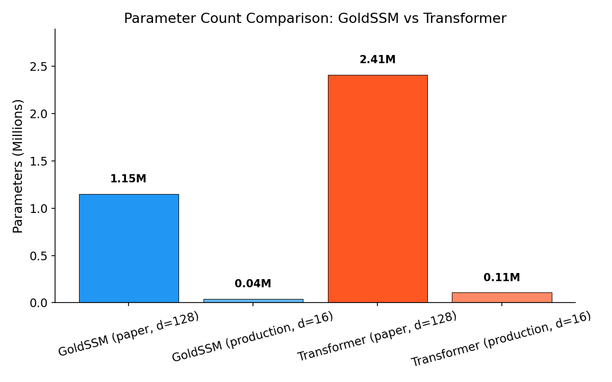
Figure 1: Parameter count comparison between GoldSSM and equivalent Transformer at $d_{\text{embed}} = 128$. GoldSSM achieves a 2.1× reduction, primarily from replacing self-attention projections with compact Mamba blocks.
7.2 VSN Regime Dependence
A permutation test (1,000 shuffles) on VSN weight vectors from the short stream confirms that feature weights are statistically dependent on regime label ($p < 0.0001$). The three most regime-variable features are the XAG-beta interaction term, the 1440-bar DXY correlation, and 60-minute returns. While cross-regime cosine similarity remains high (0.9999), the differences, though small in magnitude, are consistent and statistically significant.
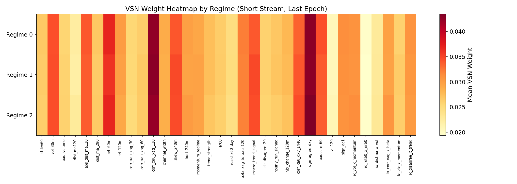
Figure 2: VSN weight distribution across regime labels. Feature weights vary systematically with regime (permutation test $p < 0.0001$), with the largest differences in cross-asset and momentum features.
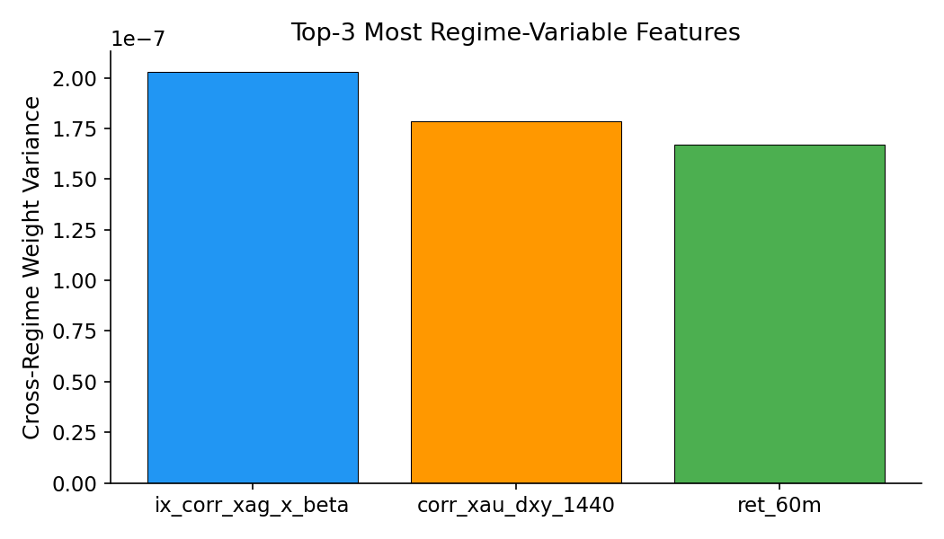
Figure 3: Top features ranked by cross-regime VSN weight variance. XAG-beta interaction, DXY correlation, and 60-minute returns show the strongest regime dependence.
7.3 Stream Gating
All four stream gates differ significantly from uniform weighting (one-sample $t$-test, $p < 0.001$ for all streams). The long stream receives the highest mean gate value (1.040), suggesting the model allocates slightly more representational weight to the 4-hour context. Gate value ranges are modest (0.02 to 0.06), indicating that gating provides fine adjustment rather than aggressive stream suppression.
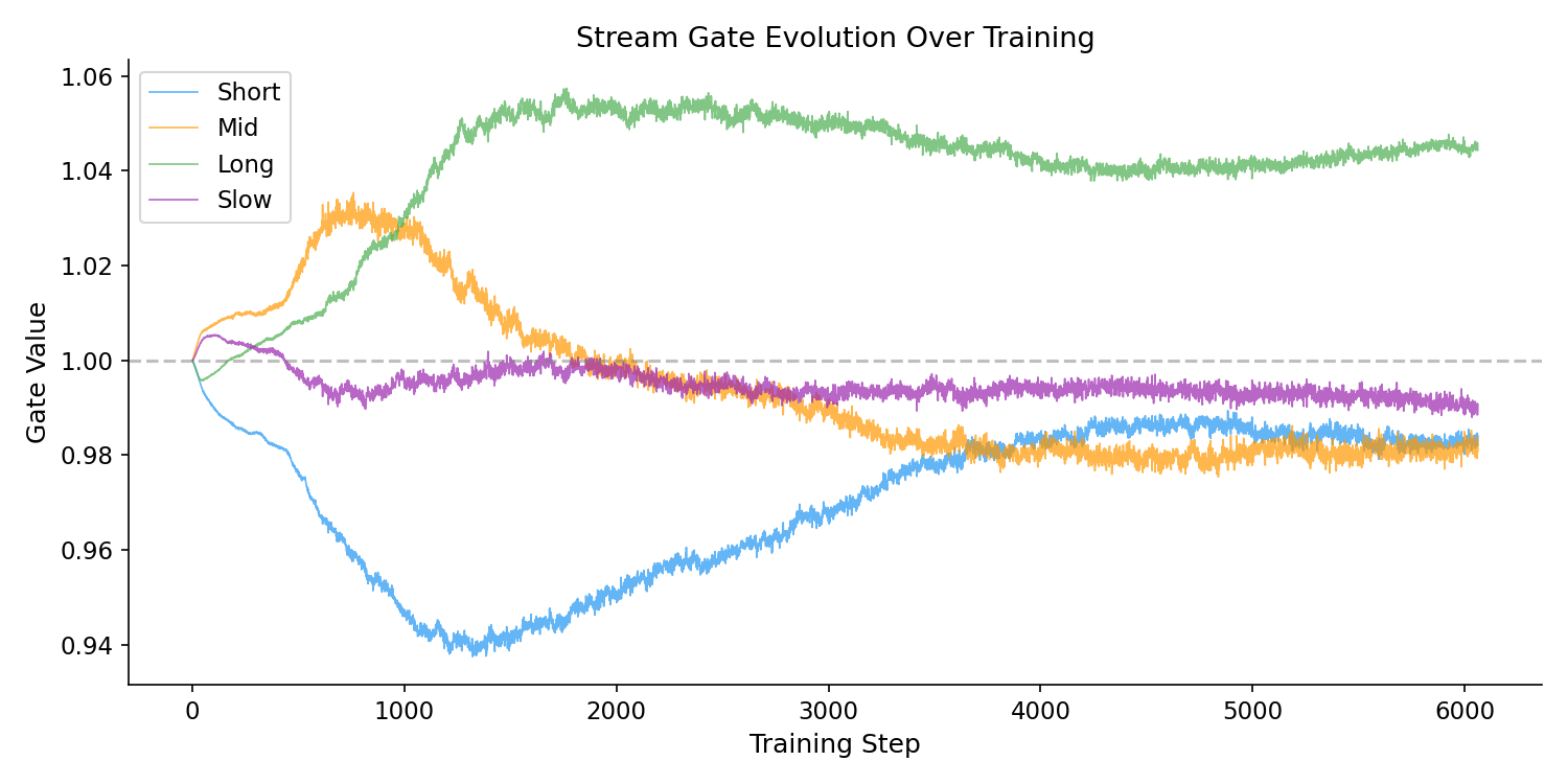
Figure 4: Stream gate values across evaluation samples. All four streams deviate significantly from uniform ($p < 0.001$), with the long stream (4h) receiving the highest mean gate weight. The narrow range (0.02–0.06) indicates fine-grained rather than binary stream selection.
7.4 Temporal Attention Pooling
TAP entropy across all four streams is 1.0, indicating that the learned queries currently distribute attention uniformly across the encoded sequence. In effect, TAP is behaving as mean pooling rather than concentrating on a sparse subset of informative bars as the architecture is designed to do. This is likely a consequence of insufficient training epochs: the queries have not yet differentiated. Longer training schedules or explicit sparsity encouragement (e.g., entropy regularisation on the attention weights) may be needed to realise the theoretical benefit of selective temporal summarisation.
7.5 Noise Robustness
Output sensitivity to input perturbation scales linearly with noise magnitude: $L_2$ distance of 0.0011 at $\sigma = 0.01$, rising to 0.052 at $\sigma = 0.50$. The near-proportional relationship and small absolute magnitudes suggest the model has not memorised bar-level patterns and responds smoothly to input variation. The noise-consistency regularisation described in Section 6 appears to be functioning as intended.
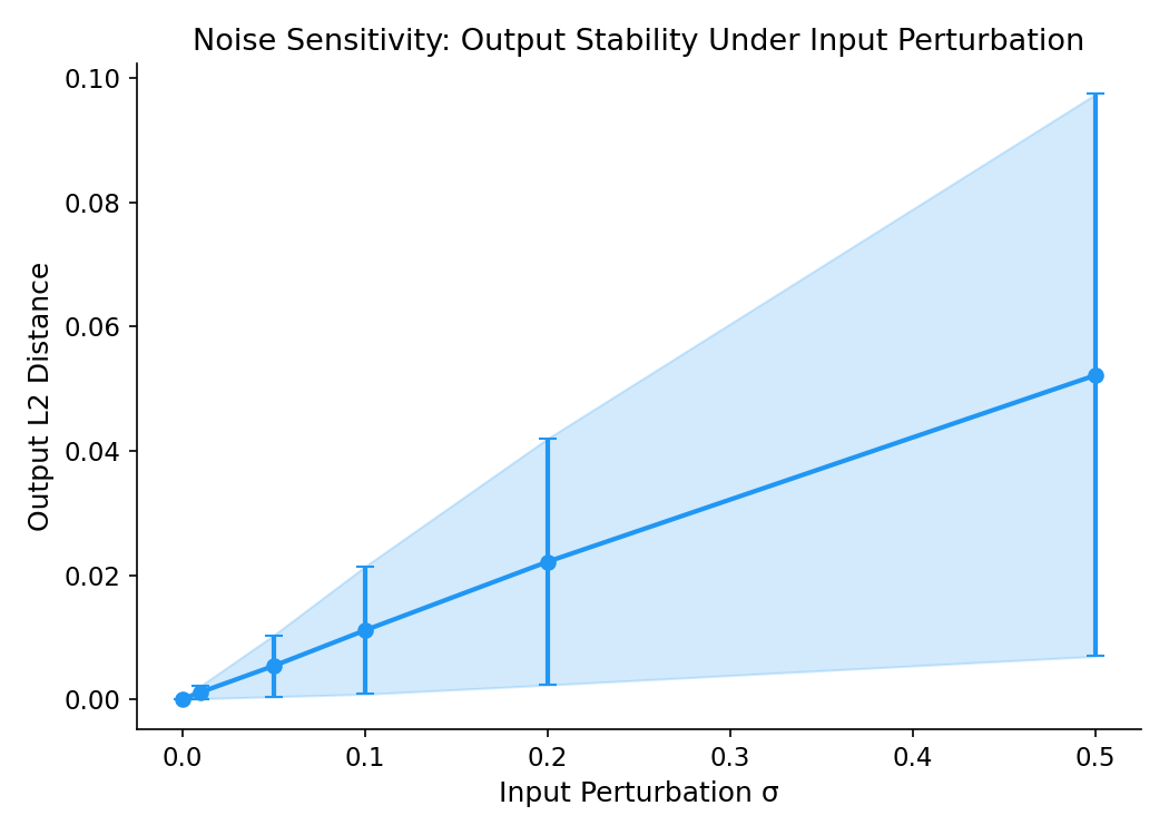
Figure 5: Output $L_2$ distance as a function of input noise standard deviation $\sigma$. The near-linear relationship confirms that the model's predictions degrade gracefully under input perturbation rather than exhibiting the sharp sensitivity characteristic of overfitting.
7.6 Causal Normalisation
Comparing KL divergence between training and out-of-sample feature distributions, causal rolling normalisation reduces distribution shift for 11 of 12 testable features, with a mean reduction of 78.6%. The largest improvements appear in volatility and volume features (stdev60: 83.6% reduction, xau_volume: 96.9%). The single feature that did not improve (er60, efficiency ratio) has an approximately stationary distribution by construction, confirming that the dual-path normalisation scheme (Section 6.1) correctly assigns stationary features to the static path.
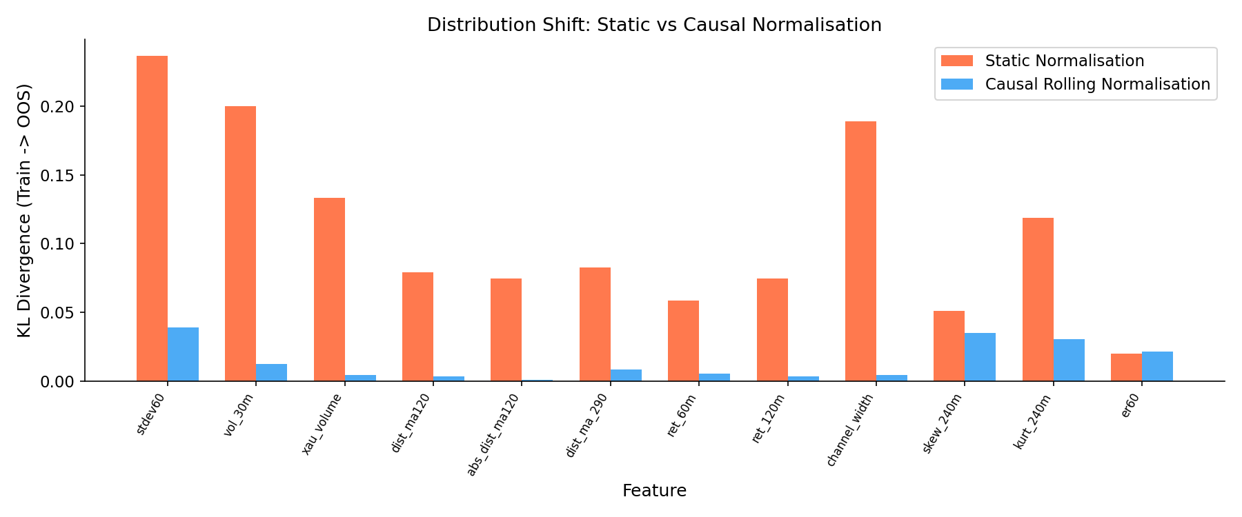
Figure 6: KL divergence between training and out-of-sample feature distributions, with and without causal rolling normalisation. 11 of 12 features show reduced distribution shift, with mean improvement of 78.6%.
8. Conclusion
GoldSSM addresses three limitations of Transformer architectures for intraday financial forecasting. Replacing quadratic self-attention with linear-time selective state space scanning enables 12-hour context windows (720 M1 bars) that would be computationally prohibitive for standard Transformers. The Variable Selection Network provides dynamic, regime-aware feature weighting at every bar, replacing the static feature treatment inherent in Transformer encoders. Learned Temporal Attention Pooling concentrates summary capacity on the sparse subset of bars that carry directional information rather than averaging across a sequence dominated by noise.
Four parallel Mamba streams with adaptive gating address the variable lookback problem directly. GoldSSM maintains simultaneous views at 1-hour, 2-hour, 4-hour, and 12-hour horizons, with learned gating that redistributes emphasis as market conditions shift. Zero-initialisation of the gating network ensures that adaptive weighting emerges only when supported by training evidence.
At approximately 1.15 million parameters ($d_{\text{embed}} = 128$), GoldSSM achieves a 2.1× reduction relative to the equivalent Transformer baseline with comparable layer depth and embedding dimension. This reduction follows from architecture, not aggressive pruning: the Mamba block's $O(d \cdot N)$ parameter scaling with $N = 8$ is inherently more compact than the $O(d^2)$ scaling of Transformer self-attention and feed-forward layers. The smaller model is less prone to overfitting on the limited, non-stationary datasets characteristic of financial machine learning. However, the parameter advantage does not currently translate into inference speed: at $T = 720$, PyTorch's highly optimised attention kernels give the Transformer a substantial wall-clock advantage (Section 5.1). The theoretical $O(T)$ scaling of SSMs is expected to become practically relevant at longer sequence lengths as Mamba kernel implementations mature.
Noise-consistency regularisation and causal normalisation complete the design. They target the central difficulty of training on M1 financial data: extremely low signal-to-noise ratio, uninformative majority bars, and continuously shifting feature distributions. Penalising sensitivity to small input perturbations and normalising features relative to their recent regime-specific distribution discourages memorisation of bar-level noise while preserving the ability to detect genuine regime-level structure.
Every architectural choice in GoldSSM is grounded in the statistical properties of financial time series rather than general-purpose sequence modelling considerations. The model is more expressive (adaptive feature selection, adaptive temporal weighting, adaptive memory horizon), more parameter-efficient (linear theoretical complexity, 2.1× fewer parameters), and better regularised (noise-consistency, causal normalisation) than the Transformer baseline it replaces. Empirical validation (Section 7) confirms the statistical claims — regime-dependent feature selection, non-uniform stream gating, noise robustness, and effective causal normalisation — while identifying areas for further work, including TAP query specialisation and closing the wall-clock gap with optimised Mamba kernels.
References
- Gu, A. and Dao, T. (2023). “Mamba: Linear-Time Sequence Modeling with Selective State Spaces.” arXiv preprint arXiv:2312.00752.
- Lim, B., Arík, S. Ö., Loeff, N., and Pfister, T. (2021). “Temporal Fusion Transformers for Interpretable Multi-horizon Time Series Forecasting.” International Journal of Forecasting, 37(4), 1748–1764.
- Zhou, H., Zhang, S., Peng, J., Zhang, S., Li, J., Xiong, H., and Zhang, W. (2021). “Informer: Beyond Efficient Transformer for Long Sequence Time-Series Forecasting.” Proceedings of the AAAI Conference on Artificial Intelligence, 35(12), 11106–11115.
- Hochreiter, S. and Schmidhuber, J. (1997). “Long Short-Term Memory.” Neural Computation, 9(8), 1735–1780.
- Vaswani, A., Shazeer, N., Parmar, N., Uszkoreit, J., Jones, L., Gomez, A. N., Kaiser, L., and Polosukhin, I. (2017). “Attention Is All You Need.” Advances in Neural Information Processing Systems, 30.
- Gu, A., Goel, K., and Ré, C. (2022). “Efficiently Modeling Long Sequences with Structured State Spaces.” International Conference on Learning Representations (ICLR).