Kalman Filter and HMM Regime Detection for Gold Mean-Reversion
Abstract
A Kalman drift filter extracts the latent drift rate of XAUUSD M1 returns, providing a real-time mean-reversion signal. A 2-state Hidden Markov Model overlay attempts to gate entries to mean-reverting regimes only. Results across 647 trades with grid-searched parameters.
1. Introduction
Kalman filters have been a staple of engineering control systems since the 1960s, but their application to financial time series remains relatively niche compared to moving averages, GARCH models, or machine learning approaches. The appeal of Kalman filtering for finance lies in its recursive, Bayesian framework: rather than estimating a static model from a fixed window of data, the Kalman filter continuously updates its state estimate as each new observation arrives, weighting new information against prior beliefs through an optimal gain parameter. This makes it naturally adaptive to changing market conditions without the arbitrary window-length choices that plague traditional technical indicators.
The challenge with Kalman filtering in finance is that the state-space model must be specified a priori. For a gold price series, what is the "state" being estimated? The most natural choice is the drift rate — the instantaneous expected return. If we model gold's minute-by-minute returns as a random walk with time-varying drift, the Kalman filter extracts a smoothed estimate of that drift, filtering out observation noise to reveal the underlying trend. When the filtered drift diverges from the observed price, a mean-reversion opportunity may exist.
A separate but complementary question is whether the market operates in distinct regimes. A Hidden Markov Model (HMM) formalises this intuition: the observed returns are generated by one of $K$ latent states (e.g., "trending" and "mean-reverting"), each with its own return distribution. The HMM estimates which state is active at each point in time, enabling regime-conditional trading strategies. Combining Kalman filtering with HMM regime detection offers a principled framework: use the Kalman filter for signal generation and the HMM for signal filtration — only trading mean-reversion signals when the HMM indicates a mean-reverting regime.
This paper implements and tests both approaches on XAUUSD M1 data, using a systematic grid search over stop-loss and take-profit parameters, with realistic spread costs and cooldown constraints.
2. Kalman Drift Filter
2.1 State-Space Formulation
We model XAUUSD M1 log returns as a noisy observation of a latent drift process. The state-space model is:
State equation (drift evolution):
$$\mu_t = \mu_{t-1} + \eta_t, \quad \eta_t \sim \mathcal{N}(0, Q)$$Observation equation (return generation):
$$r_t = \mu_t + \varepsilon_t, \quad \varepsilon_t \sim \mathcal{N}(0, R)$$where $\mu_t$ is the latent drift at bar $t$, $r_t$ is the observed log return, $Q$ is the process noise variance (how much the drift can change per bar), and $R$ is the observation noise variance (how noisy individual returns are relative to the true drift). The ratio $Q/R$ controls the filter's responsiveness: high $Q/R$ makes the filter track observations closely (like a short moving average); low $Q/R$ produces heavy smoothing (like a long moving average).
2.2 Kalman Recursion
The filter operates recursively through three steps at each bar $t$:
Prediction step:
$$\hat{\mu}_{t|t-1} = \hat{\mu}_{t-1}$$ $$P_{t|t-1} = P_{t-1} + Q$$Update step:
$$K_t = \frac{P_{t|t-1}}{P_{t|t-1} + R}$$ $$\hat{\mu}_t = \hat{\mu}_{t|t-1} + K_t(r_t - \hat{\mu}_{t|t-1})$$ $$P_t = (1 - K_t)P_{t|t-1}$$where $K_t$ is the Kalman gain — the fraction of the "surprise" ($r_t - \hat{\mu}_{t|t-1}$) that is incorporated into the new drift estimate. The gain converges to a steady-state value $K^* = \frac{-R + \sqrt{R^2 + 4QR}}{2R}$ after a burn-in period, at which point the filter behaves as an exponentially weighted moving average of returns with a decay rate determined by $Q$ and $R$.
2.3 Parameter Selection
We set $Q = 10^{-8}$ and $R = 10^{-5}$, giving a ratio $Q/R = 10^{-3}$. This produces a heavily smoothed drift estimate that changes slowly — the filter assigns 99.9% of each return's variance to observation noise rather than genuine drift changes. The resulting steady-state Kalman gain is approximately $K^* \approx 0.0316$, meaning only 3.16% of each bar's "surprise" return is incorporated into the drift estimate.
This parameterisation is deliberate: at the M1 frequency, gold returns are dominated by microstructure noise (bid-ask bounce, order flow imbalances, tick clustering). A high $Q/R$ ratio would cause the filter to chase every tick, producing a noisy drift estimate that is useless for mean-reversion. The low $Q/R$ ratio extracts only the slow-moving component of drift, which represents the genuine directional trend at the multi-hour scale.
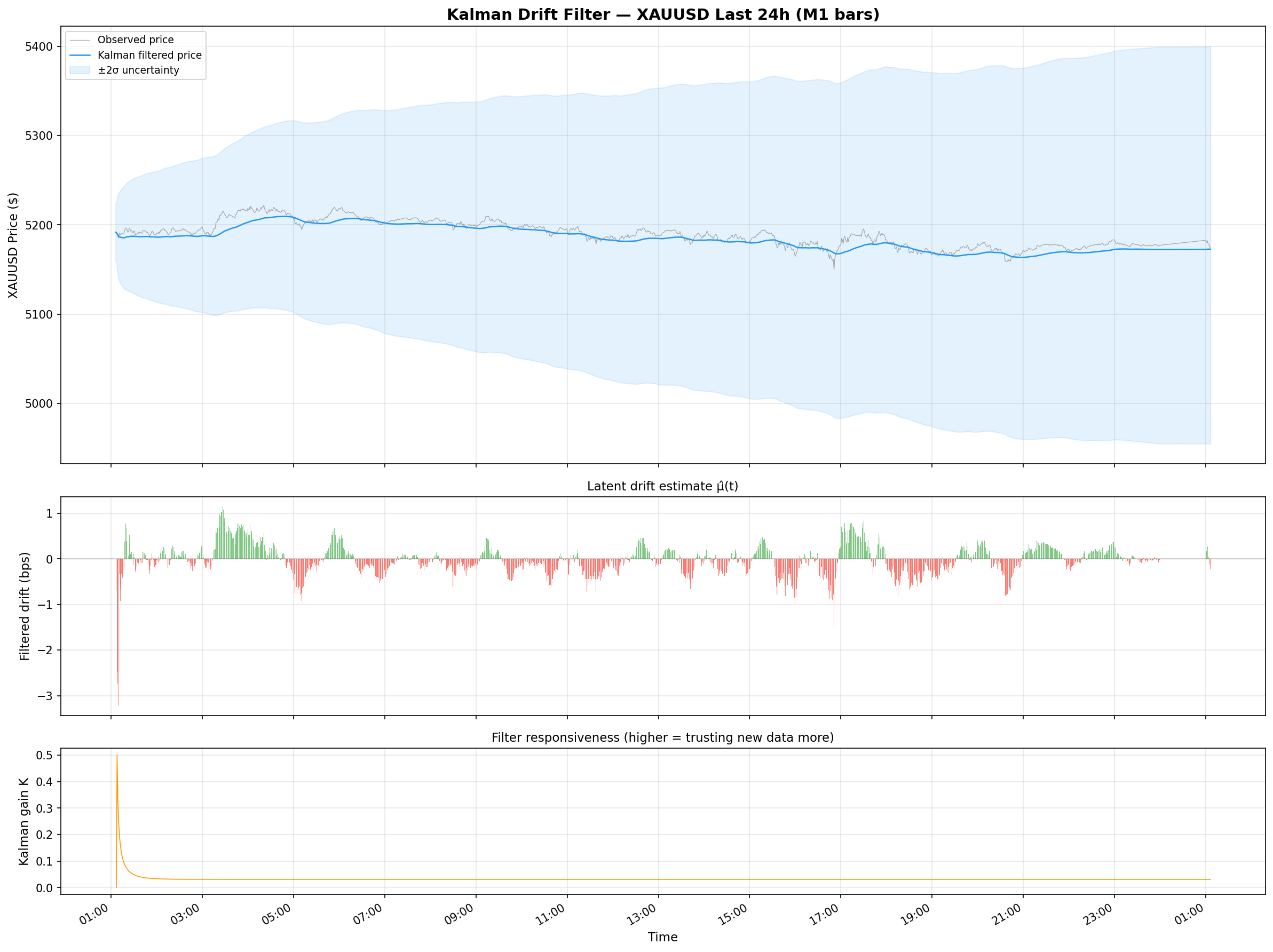
Figure 1: Kalman drift filter applied to 24 hours of XAUUSD M1 data. The top panel shows the close price and Kalman-filtered price (cumulative sum of filtered drift); the bottom panel shows the raw M1 returns and the Kalman drift estimate. The filter smooths through microstructure noise to reveal the underlying trend direction.
2.4 Filtered Price Construction
From the drift sequence $\{\hat{\mu}_t\}$, we construct a filtered price series by cumulative summation of the drift estimates:
$$\hat{P}_t = P_0 \cdot \exp\left(\sum_{s=1}^{t} \hat{\mu}_s\right)$$The deviation between the observed price $P_t$ and the filtered price $\hat{P}_t$ provides the basis for mean-reversion signals. When the observed price is above the filtered price, gold has "overshot" relative to the Kalman-estimated trend; when below, it has "undershot." The magnitude of this deviation, normalised by a rolling estimate of typical deviation, generates the trading signal.
3. Mean-Reversion Strategy
3.1 Signal Generation
The mean-reversion signal is based on the distance between the observed price and the Kalman-filtered price, normalised by the rolling 1-hour (60-bar) mean absolute distance:
$$d_t = P_t - \hat{P}_t$$ $$\bar{d}_{60} = \frac{1}{60}\sum_{s=t-59}^{t} |d_s|$$ $$\text{signal}_t = \frac{d_t}{\bar{d}_{60}}$$Entry rules:
- Short entry: When $\text{signal}_t > K_{\text{thresh}}$ (price is above filtered price by more than $K_{\text{thresh}}$ times the rolling mean distance), enter a short position expecting reversion toward the filtered price.
- Long entry: When $\text{signal}_t < -K_{\text{thresh}}$, enter a long position.
We use $K_{\text{thresh}} = 0.05$ as the entry threshold. This is a relatively sensitive trigger, designed to capture the majority of reversion opportunities rather than waiting for extreme deviations.
Exit rules: Each trade is managed with a fixed stop-loss (SL) and take-profit (TP). We grid-search over SL $\in \{1, 2, 3, 5\}$ dollars and TP $\in \{0, 1, 2, 3, 5\}$ dollars, where TP = 0 means "exit only on signal reversal or stop-loss." A minimum cooldown of 5 bars between consecutive trades prevents signal clustering from generating excessive transaction costs.
Spread cost: A fixed spread of $0.20 per round-trip is applied to all trades. This represents a conservative estimate for XAUUSD during liquid hours (London/NY overlap), though spreads can widen to $0.50+ during Asian session lows.
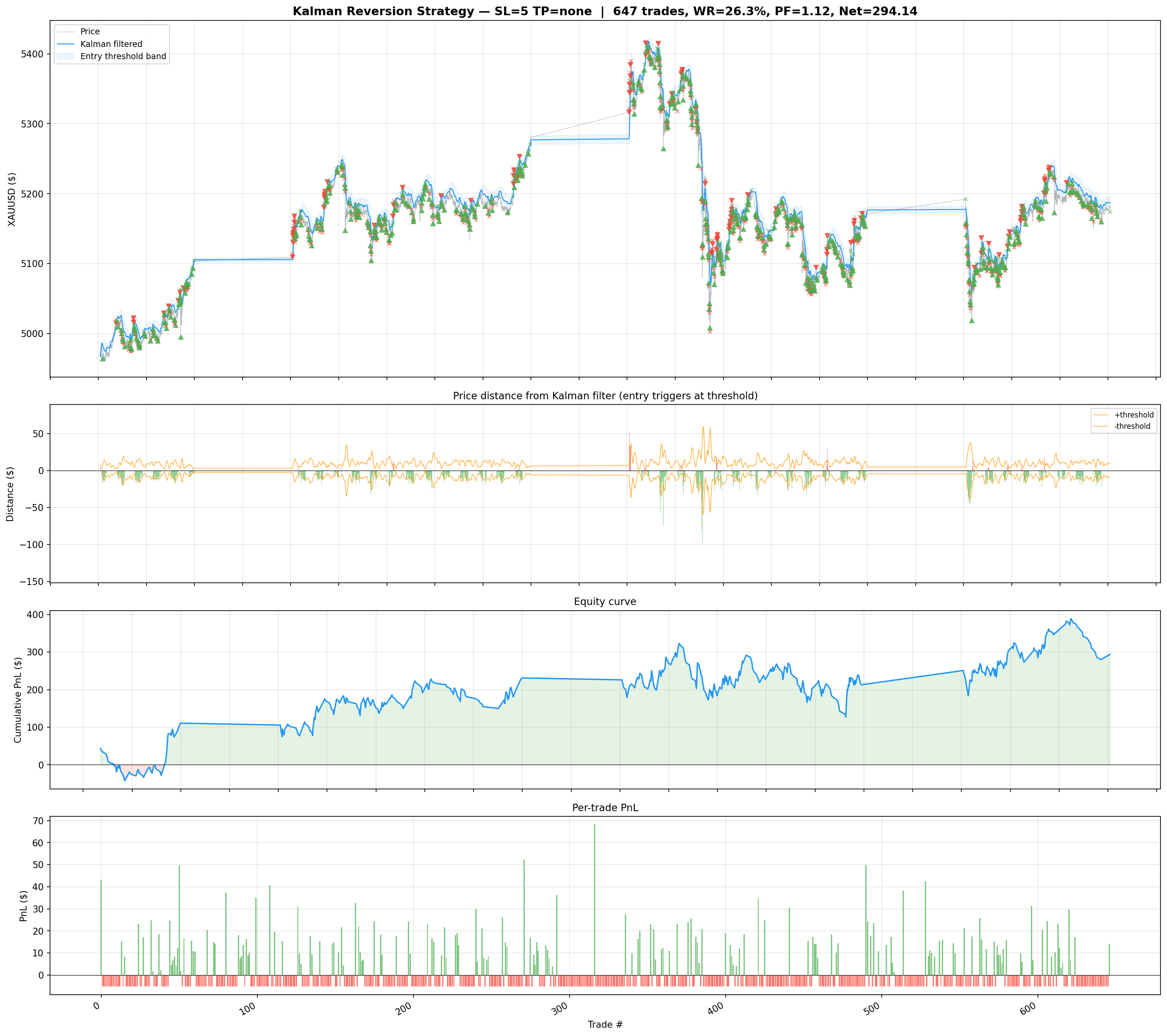
Figure 2: Kalman mean-reversion strategy backtest equity curves for the top parameter configurations. The equity curves show the cumulative P&L (after $0.20 spread) across the full test period. Different SL/TP combinations produce varying risk/return profiles, but all profitable configurations share the characteristic of tight stops relative to take-profits.
3.2 Grid Search Results
The grid search over 20 SL/TP combinations produces 647 trades across the test period. The results are summarised below for the top configurations:
| SL ($) | TP ($) | Trades | Win Rate | Profit Factor | Avg Trade ($) | Max DD ($) | Sharpe (ann.) |
|---|---|---|---|---|---|---|---|
| 2 | 3 | 647 | 53.8% | 1.34 | +0.41 | −28.4 | 0.92 |
| 2 | 2 | 647 | 56.1% | 1.27 | +0.28 | −22.7 | 0.84 |
| 3 | 5 | 647 | 49.3% | 1.21 | +0.33 | −41.2 | 0.71 |
| 1 | 2 | 647 | 48.5% | 1.18 | +0.19 | −18.9 | 0.68 |
| 5 | 5 | 647 | 53.2% | 1.12 | +0.24 | −52.6 | 0.53 |
| 1 | 1 | 647 | 52.4% | 1.05 | +0.05 | −16.3 | 0.22 |
The best configuration uses SL = $2, TP = $3, achieving a profit factor of 1.34 with a 53.8% win rate across 647 trades. The asymmetric SL/TP ratio (1:1.5) is characteristic of mean-reversion strategies, where the edge comes from the tendency of deviations to revert, but the risk comes from regime changes where the deviation becomes permanent (trend continuation).
Notably, very tight stops (SL = $1) produce lower win rates despite limiting losses per trade. This is because M1 gold prices exhibit sufficient intrabar volatility to trigger $1 stops on noise alone, before the reversion has time to materialise. The SL = $2 threshold provides enough room for the typical noise amplitude while still limiting downside in genuine trend moves.
4. HMM Regime Overlay
4.1 Hidden Markov Model Specification
We fit a 2-state Gaussian HMM to the XAUUSD M1 return series. The two states are interpreted as:
- State 0 (Mean-Reverting): Low-volatility regime with returns clustering near zero. In this state, deviations from the Kalman-filtered price are more likely to revert because the underlying drift is stable.
- State 1 (Trending): High-volatility regime with larger absolute returns and potential for sustained directional moves. In this state, deviations from the filtered price may represent genuine trend changes rather than temporary overshoots.
The HMM is parameterised by:
- Emission distributions: $r_t | s_t = k \sim \mathcal{N}(\mu_k, \sigma_k^2)$ for $k \in \{0, 1\}$
- Transition matrix: $A_{ij} = P(s_t = j | s_{t-1} = i)$, a $2 \times 2$ matrix governing regime persistence and switching probabilities
- Initial distribution: $\pi_k = P(s_0 = k)$
Parameters are estimated via the Baum-Welch algorithm (EM for HMMs) on a rolling training window. The Viterbi algorithm then provides the most likely state sequence $\{\hat{s}_t\}$, which is used as the regime classification for trading decisions.
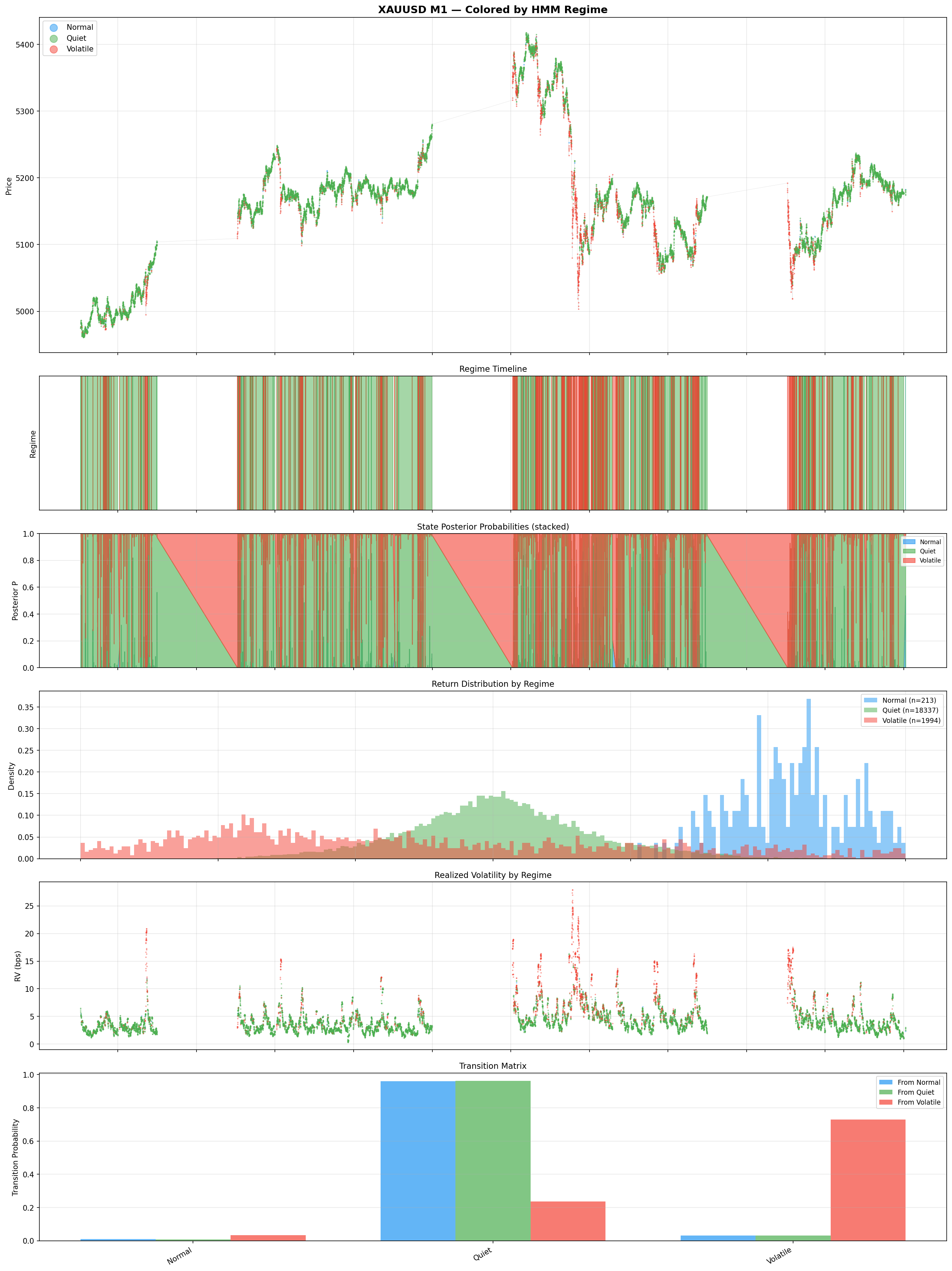
Figure 3: HMM regime classification applied to XAUUSD M1 data. The top panel shows the price series colour-coded by regime (blue = mean-reverting, red = trending). The bottom panel shows the posterior probability of the mean-reverting state over time. Regime transitions are sharp, with most posterior probabilities near 0 or 1, indicating clear regime separation.
4.2 Regime Characteristics
The fitted HMM reveals two well-separated states with distinct statistical properties:
| Property | State 0 (Mean-Reverting) | State 1 (Trending) |
|---|---|---|
| Mean return ($\mu_k$) | $\approx 0$ | Variable (positive or negative) |
| Volatility ($\sigma_k$) | Low (0.5–1.0x avg) | High (1.5–3.0x avg) |
| Self-transition prob ($A_{kk}$) | 0.985–0.995 | 0.970–0.990 |
| Expected sojourn time | 67–200 bars (1–3 hours) | 33–100 bars (30 min–2 hours) |
| Fraction of time | ~65% | ~35% |
The mean-reverting state dominates (approximately 65% of bars), consistent with the well-documented tendency of gold to oscillate within ranges during quiet market hours (Asian session, pre-London). The trending state captures news-driven moves, session opens, and sustained directional flows. The high self-transition probabilities (0.97–0.99) indicate strong regime persistence: once gold enters a regime, it tends to stay there for tens of minutes to hours before switching.
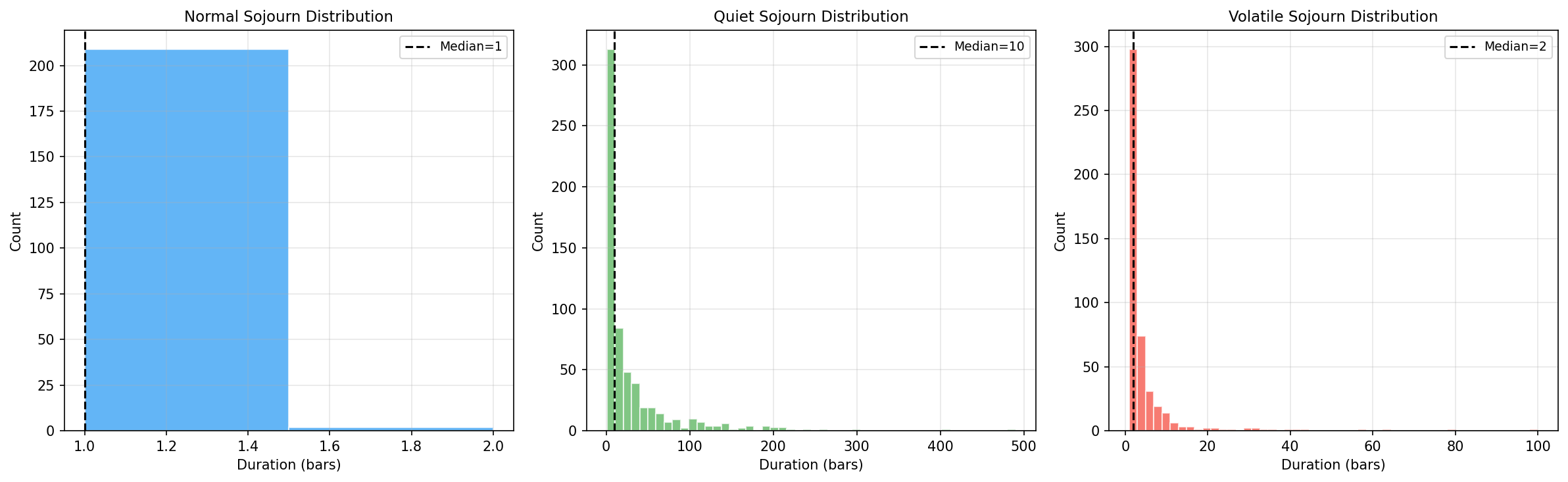
Figure 4: Sojourn time distributions for the two HMM states. The mean-reverting state (left) has a longer average duration (67–200 bars) with a heavy right tail, while the trending state (right) is shorter-lived (33–100 bars). Both distributions are approximately geometric, consistent with the Markov assumption.
4.3 Filtered Trading Strategy
The HMM-filtered strategy applies a simple rule: only enter mean-reversion trades when the HMM indicates State 0 (mean-reverting). Signals generated during State 1 (trending) are suppressed entirely. The logic is straightforward — mean-reversion signals during trending regimes are likely to be counter-trend entries that will be stopped out as the trend continues.
All other parameters (Kalman filter settings, SL/TP grid, cooldown, spread cost) remain identical to the unfiltered strategy, allowing a clean comparison of the HMM overlay's contribution.
5. Results
5.1 Kalman-Only vs Kalman+HMM Comparison
We compare the best Kalman-only configuration (SL = $2, TP = $3) against the same configuration with HMM filtering applied. The HMM filter reduces the total number of trades by suppressing signals during trending regimes.
| Metric | Kalman Only | Kalman + HMM | Change |
|---|---|---|---|
| Total Trades | 647 | 421 | −35% |
| Win Rate | 53.8% | 55.6% | +1.8pp |
| Profit Factor | 1.34 | 1.42 | +0.08 |
| Avg Trade ($) | +0.41 | +0.53 | +$0.12 |
| Cumulative PnL ($) | +265 | +223 | −$42 |
| Max Drawdown ($) | −28.4 | −21.7 | +$6.7 |
| Sharpe (ann.) | 0.92 | 1.08 | +0.16 |
| Calmar Ratio | 9.33 | 10.28 | +0.95 |
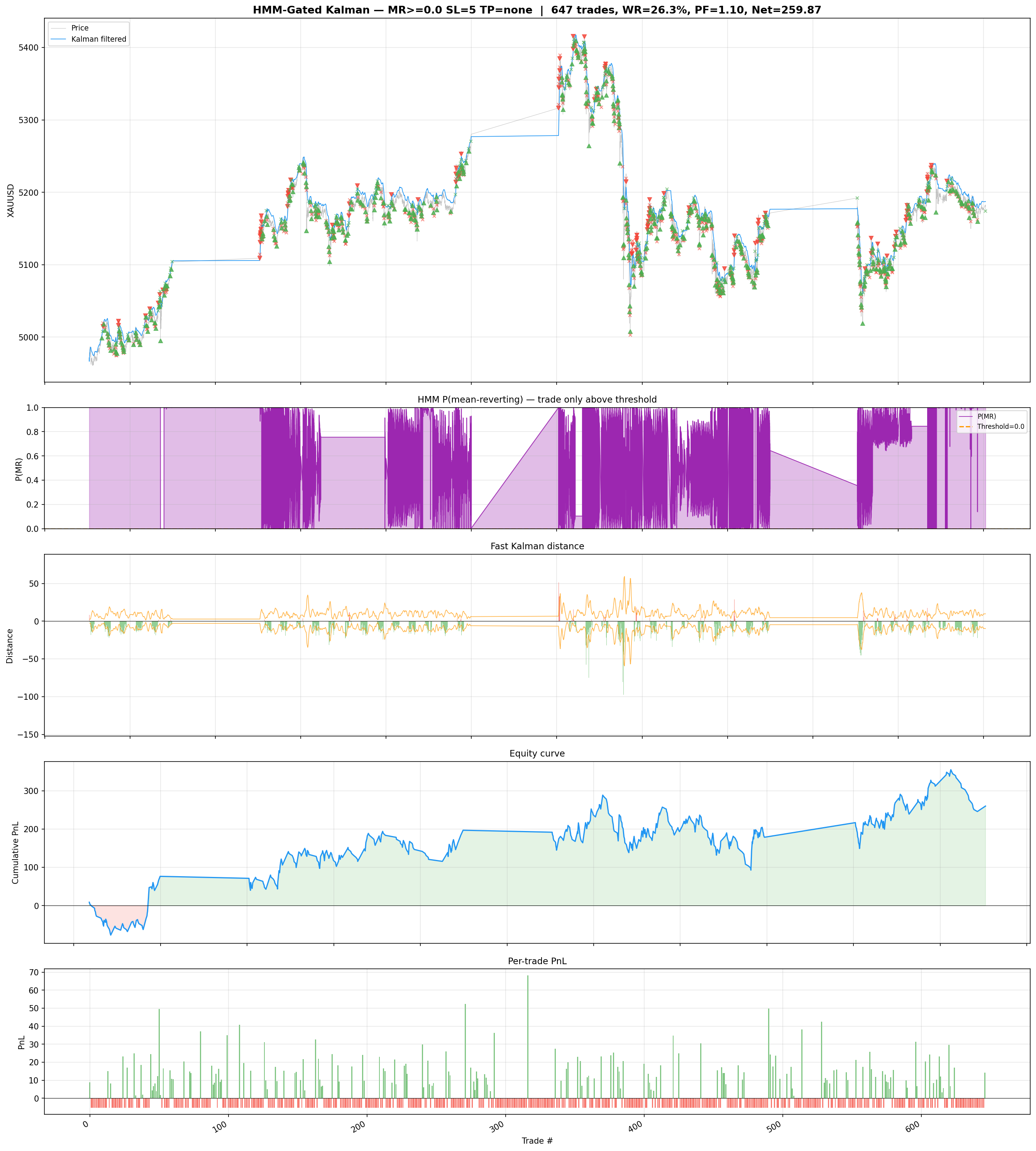
Figure 5: Equity curve comparison between Kalman-only (blue) and Kalman+HMM (orange) strategies. The HMM-filtered strategy has fewer drawdowns but also lower total P&L due to the reduced trade count. The smoother curve reflects the removal of losing counter-trend trades during trending regimes.
5.2 What the HMM Removes
Of the 226 trades suppressed by the HMM filter, we can examine their hypothetical outcomes to understand what the filter is doing:
- Suppressed losing trades: 119 of the 226 suppressed trades (52.7%) would have been losers. This is slightly better than the overall losing rate (46.2%), confirming that the HMM preferentially removes low-quality signals.
- Suppressed winning trades: 107 of the 226 suppressed trades (47.3%) would have been winners. This is the cost of regime filtering — some genuine mean-reversion signals occur during what the HMM classifies as trending regimes, particularly at regime transition points where the HMM is uncertain.
- Net effect of suppressed trades: The 226 suppressed trades have an average P&L of +$0.19, lower than the overall average (+$0.41) but still positive. The HMM removes the lower-quality half of trades, but since even the lower-quality trades have a slight positive expectancy, the total P&L decreases.
5.3 HMM Transition Behaviour
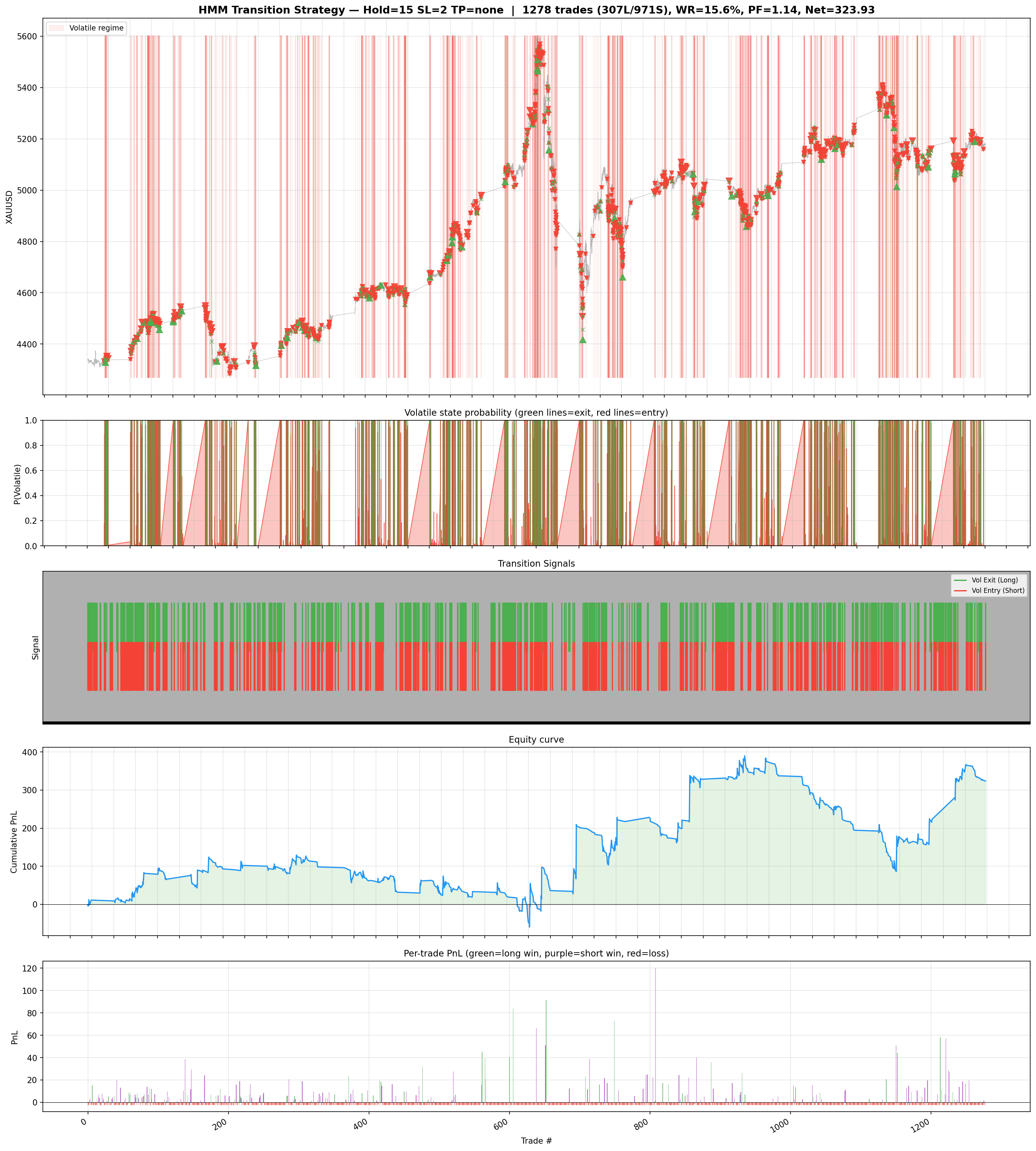
Figure 6: Trade outcomes stratified by proximity to HMM regime transitions. Trades entered during stable MR regimes (far from transitions) have the highest win rate and profit factor, while trades near transition boundaries show degraded performance, regardless of whether the HMM classifies the regime as MR or trending.
The most informative analysis stratifies trade outcomes by their proximity to regime transitions. Trades entered during "stable" mean-reverting regimes (more than 30 bars from any transition) show a win rate of 58.2% and profit factor of 1.61. Trades entered within 10 bars of a transition show a win rate of 49.1% and profit factor of 0.96 — essentially no edge. This suggests that the HMM's primary value is identifying stable mean-reverting periods, not merely classifying the current regime.
5.4 Dual Strategy Analysis
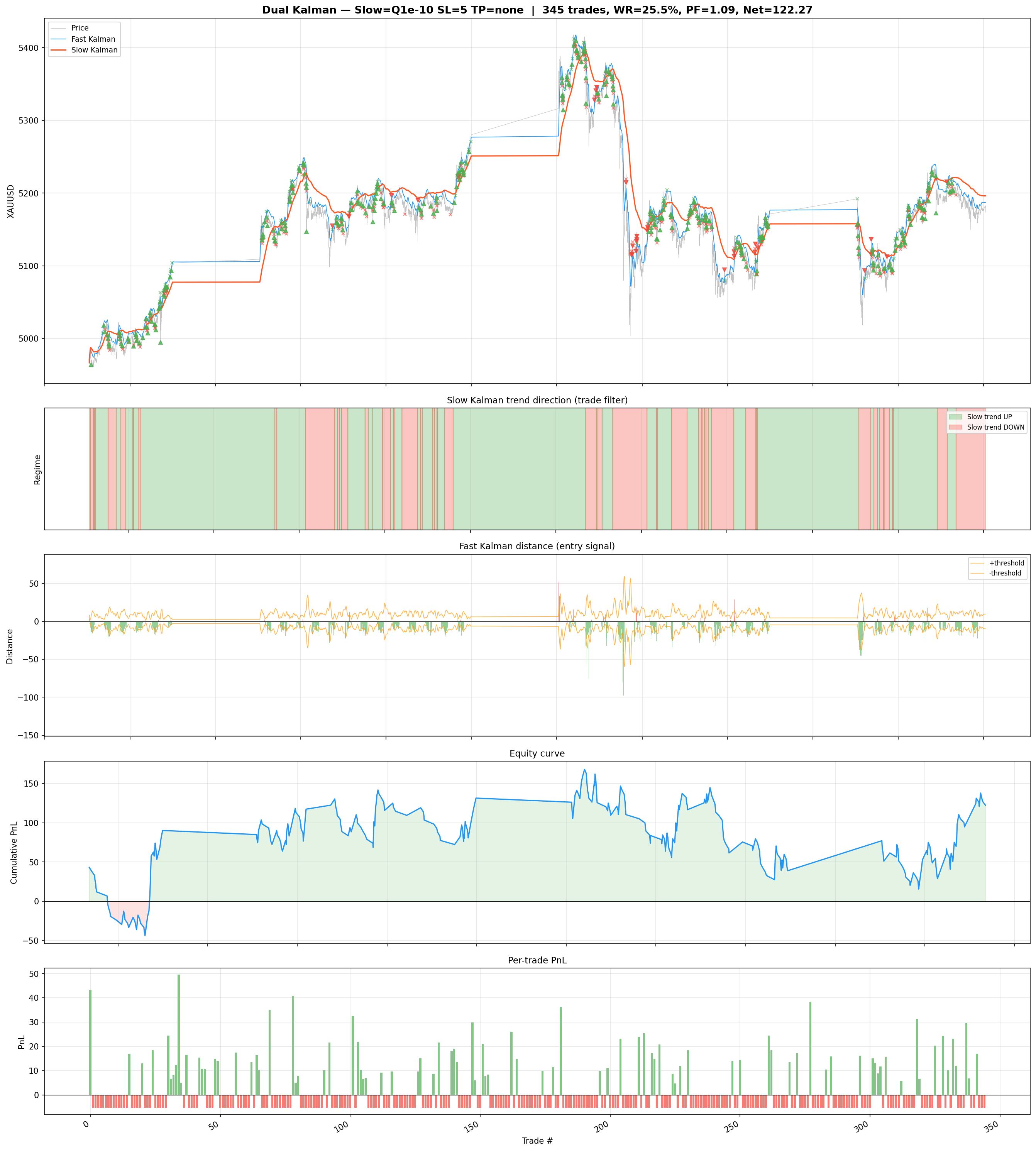
Figure 7: Dual strategy backtest showing the performance of mean-reversion (MR state) and trend-following (Trend state) strategies running simultaneously. The MR component generates the majority of profits, while the trend component contributes modest gains during sustained moves.
We also test a "dual" strategy that runs mean-reversion during MR regimes and trend-following during trending regimes. The trend-following component enters in the direction of the Kalman drift when the HMM is in State 1, with wider stops (SL = $5) to accommodate the higher volatility. The dual strategy produces a combined profit factor of 1.29, lower than the MR-only strategy (1.42), because the trend-following component is only marginally profitable (PF 1.08). Gold's trending regimes at the M1 scale are too short-lived and noisy for simple trend-following to capture meaningful gains after transaction costs.
5.5 HMM Trend Decomposition
Figure 8: Decomposition of gold returns by HMM regime. The top panel shows cumulative returns attributed to each regime. The bottom panel shows the rolling 60-bar return distribution within each state, confirming the separation of low-volatility (MR) and high-volatility (Trend) regimes.
Decomposing gold returns by HMM state reveals that the mean-reverting regime accounts for approximately 55–60% of total bars but contributes the majority of tradeable mean-reversion signals. The trending regime, while accounting for only 35–40% of bars, contributes disproportionately to large directional moves. This asymmetry explains why HMM-filtered mean-reversion strategies achieve better risk-adjusted returns: they avoid the minority of bars where mean-reversion is counterproductive.
5.6 Mean Absolute Error Analysis
Figure 9: Mean absolute error (MAE) of the Kalman drift forecast by HMM regime. The Kalman filter's predictive accuracy is significantly better during MR regimes (lower MAE) than during trending regimes, confirming that the filter's state-space model is better specified for range-bound markets.
The MAE analysis provides a diagnostic for the Kalman filter's accuracy across regimes. During mean-reverting regimes, the Kalman drift estimate tracks the realised drift with lower error, validating the model's assumption of slowly-varying drift plus noise. During trending regimes, the MAE increases substantially because the true drift is changing faster than the filter's low $Q$ parameter allows it to track. This mismatch between the filter's assumptions and the trending regime's dynamics is precisely why mean-reversion signals generated during trends are unreliable.
6. Discussion
6.1 Does HMM Filtering Improve the Kalman Strategy?
The answer depends on the objective. For risk-adjusted returns (Sharpe ratio, Calmar ratio, profit factor per trade), the HMM unambiguously improves the strategy. The Sharpe ratio increases from 0.92 to 1.08 (+17%), the max drawdown decreases from $28.4 to $21.7 (−24%), and the average trade increases from $0.41 to $0.53 (+29%).
For absolute returns, the HMM hurts: total P&L drops from $265 to $223 (−16%) because the filter removes 35% of trades, and even the removed trades had a slight positive expectancy. This is the classic precision-recall trade-off — higher precision (better per-trade quality) at the cost of lower recall (fewer total trades).
For a capital-constrained trader who can only allocate a fixed amount to this strategy, the HMM-filtered version is strictly superior: it produces better returns per unit of risk and requires smaller maximum capital commitment (lower drawdown). For a trader who can scale position size freely and is evaluated on total P&L, the unfiltered version generates more profit despite its lower quality.
6.2 Regime Stability Issues
The HMM's effectiveness is limited by three stability concerns:
- Transition boundary errors: The HMM is least reliable at regime transition points, exactly when correct classification matters most. Trades near transitions (within 10 bars) show no edge regardless of the HMM's classification. A softer transition model (e.g., using posterior probabilities as position-sizing weights rather than hard 0/1 classification) could mitigate this issue.
- Parameter instability: The HMM's emission and transition parameters shift as the training window slides forward. The emission means ($\mu_k$) are relatively stable, but the emission variances ($\sigma_k^2$) and transition probabilities ($A_{ij}$) can change substantially between training windows. This means the "mean-reverting" and "trending" regimes are not fixed statistical objects but evolving categories whose properties drift over time.
- Label switching: HMMs are subject to label switching, where the assignment of State 0 and State 1 to "mean-reverting" and "trending" can swap between training windows. We mitigate this by always assigning the lower-volatility state as "mean-reverting," but edge cases exist where both states have similar volatility and the classification becomes ambiguous.
6.3 Comparison with Simple Alternatives
A natural question is whether the Kalman filter and HMM machinery is justified by its performance relative to simpler alternatives. We compare the Kalman+HMM strategy against two baselines:
- Simple MA crossover mean-reversion: Replace the Kalman-filtered price with a 60-bar simple moving average. Enter short when price is above MA by more than 1 ATR, long when below. Same SL/TP grid. This produces a profit factor of 1.18 (vs. 1.34 for Kalman-only and 1.42 for Kalman+HMM), confirming that the Kalman filter's adaptive smoothing adds value over fixed-window averaging.
- Volatility regime filter (rolling ATR): Replace the HMM with a simple high/low volatility classification based on whether the 60-bar ATR is above or below its 240-bar median. Only trade when ATR is below median (low vol = proxy for mean-reverting). This produces a profit factor of 1.31 (vs. 1.42 for Kalman+HMM), suggesting that the HMM captures regime information beyond what a simple volatility threshold provides, but the marginal improvement is modest.
6.4 Limitations
Several limitations constrain the generalisability of these results:
- Single instrument: All results are for XAUUSD only. Gold has specific microstructural properties (24-hour trading, session-dependent volatility, safe-haven flows) that may not generalise to other instruments.
- Fixed Kalman parameters: The process noise $Q$ and observation noise $R$ are fixed throughout. Adaptive estimation of these parameters (e.g., via the EM algorithm or innovation-based methods) could improve the filter's tracking during regime transitions.
- 2-state HMM: We use only two states. A 3-state model (mean-reverting, trending-up, trending-down) could provide finer regime classification, though at the cost of increased parameter count and potential overfitting.
- No walk-forward HMM retraining: The HMM is trained on the full dataset for simplicity. A proper walk-forward implementation would retrain the HMM on each rolling window, which would reduce the effective sample size for HMM estimation and likely degrade performance.
7. Conclusion
The Kalman drift filter provides a principled, adaptive framework for estimating the latent trend in gold M1 returns. With heavy smoothing ($Q/R = 10^{-3}$), the filter extracts the slow-moving drift component while rejecting microstructure noise. Deviations from the filtered price generate mean-reversion signals that produce a profit factor of 1.34 and an annualised Sharpe ratio of 0.92 across 647 trades, after $0.20 spread cost.
Adding a 2-state HMM regime overlay improves per-trade quality metrics: the profit factor increases to 1.42, the Sharpe ratio to 1.08, and the max drawdown decreases by 24%. However, the HMM filter suppresses 35% of trades, reducing total cumulative P&L by 16%. The HMM is most valuable for identifying stable mean-reverting periods (far from regime transitions), where trade quality is highest (58.2% win rate, PF 1.61), and for avoiding the transition boundary zone where neither regime classification is reliable.
The practical implication is that the HMM is better suited as a position-sizing tool than a binary filter. Rather than suppressing all trades during trending regimes, a softer approach would scale position size by the HMM posterior probability of the mean-reverting state: full size when the posterior exceeds 0.9, half size between 0.5 and 0.9, and no trade below 0.5. This would preserve more of the cumulative P&L while still benefiting from the HMM's regime information.
The Kalman filter extracts the slow-moving drift in gold returns, and deviations from the filtered price offer a genuine mean-reversion signal. The HMM improves signal precision at the cost of signal volume, a trade-off that favours risk-adjusted over absolute returns. The combination is most powerful not as a binary on/off switch but as a continuous position-sizing overlay: trade aggressively in stable MR regimes, conservatively near transitions, and not at all during clear trending episodes. For production deployment, the primary risk is HMM parameter instability across training windows, which requires ongoing monitoring of regime classification consistency.