Three Textbook Edges Meet the Spread: A Mean-Reversion Replication on Index CFDs
Abstract
We replicate three of the most-cited OHLCV-only mean-reversion edges on the instruments people actually trade (US30, US500 and NASDAQ CFDs), with a realistic spread on every entry and exit and a frozen-parameter walk-forward. Overnight gap-fade does not replicate: its famous ~90% fill rate is an artefact of tiny gaps, and gaps large enough to fade fill under half the time (only 16% for large NASDAQ gaps). The IBS effect's reported ~70% win rate collapses to ~50%, a coin flip. Connors RSI(2) is the one partial survivor, with real 57-67% win rates, but it trades too rarely to beat a trending index. After costs and out-of-sample, none of the three beats buy-and-hold. The point is not that mean reversion is fake, but that venue, costs, and out-of-sample decay separate a backtest in a paper from a position in a live account.
1. Why we ran this
Most published trading edges are reported on US cash equities, over a chosen sample, often with costs waved away and almost never with honest out-of-sample testing. The retail and semi-professional world that reads those papers does not trade that venue. It trades index CFDs, where the spread is wide and pays on every entry and exit. So we took three of the most-cited mean-reversion edges in the practitioner literature and asked a single practical question: do they survive on the instruments people actually trade, once you charge a realistic spread and validate out-of-sample?
The three are: overnight gap-fade (gaps tend to reverse, or "fill", intraday; Stübinger and Schneider, 2019), the IBS effect (Pagonidis, 2014: when a day closes near its low, the next day tends to rise), and Connors RSI(2) (Connors and Alvarez, 2008: buy a short-term oversold reading in an uptrend). We replicated all three on US30, US500 and the NASDAQ (NAS100) over five to eight years of data.
This is not a claim that the original authors were wrong on their own data. It is a narrower and more useful statement: these edges do not transfer to index CFDs net of costs, which is exactly the gap between a backtest in a paper and a position in a live account.
2. Setup
All three studies share one harness. Data is minute-resolution price bars for US30 (2020-08 to 2026-03), US500 and the NASDAQ (both 2018-05 to 2026-03), resampled to the frequency each strategy needs. The harness is causal by construction: a signal computed at one day's close is acted on at the next session's open and exited later, with no overlapping trades and nothing from the future touching the decision.
We charge the broker spread on both entry and exit. The spread on US500 and the NASDAQ is far wider than on the Dow and is the binding constraint on any high-frequency mean-reversion rule. Our cost model is, if anything, optimistic: a single representative spread per instrument, with no commission and no slippage. That matters for the direction of the conclusion. More realistic costs would only widen the gap to buy-and-hold, never close it, so an honest negative result here is a conservative one.
Every strategy is judged two ways. First on the full sample with the literature's own fixed parameters (a faithful replication). Then with a rolling walk-forward: parameters are grid-searched on a two-year training window, frozen, and applied to the next out-of-sample year, with no re-optimisation. The benchmark throughout is buy-and-hold over the identical period. We report win rate, profit factor, and performance versus buy-and-hold, and deliberately avoid quoting annualised Sharpe ratios, which are unstable and misleading on the small trade counts these strategies generate.
3. Edge 1: overnight gap-fade
In plain terms: markets close overnight, but news keeps arriving, so a market often opens at a different price from where it closed the day before. That jump is the overnight gap. "Fading" the gap means betting that it reverses: if the market gaps up at the open you sell, expecting price to drift back down toward the previous close; if it gaps down you buy. The gap is said to "fill" when price returns to the prior close, which is the outcome the fade is hoping for. The strategy is popular because, counted naively, gaps fill most of the time.
3.1 The claim
The strongest concrete version of the gap-fade claim is Stübinger and Schneider (2019), who report a mean-reverting overnight-gap statistical-arbitrage strategy on S&P 500 constituents earning around 51.5% per year. That is a high-frequency, many-stock statistical-arbitrage result, not a simple index rule, and figures like that are notoriously sensitive to costs and to the breadth of the stock universe. The simpler, more popular version, fade the gap on a single index because "gaps always fill", is largely practitioner lore. We tested the practical version: at each open, if the gap exceeds a size threshold, fade it, taking profit if price returns to the prior close and exiting at the day's close otherwise.
3.2 The aggregate fill rate is misleading
The statistic usually cited in support of the strategy is the aggregate gap-fill rate: 91.4% on US30, 89.8% on US500, and 88.9% on the NASDAQ. These figures are accurate, but they are uninformative for a fade strategy, because they are dominated by tiny gaps. Disaggregating the fill rate by gap size reverses the conclusion.
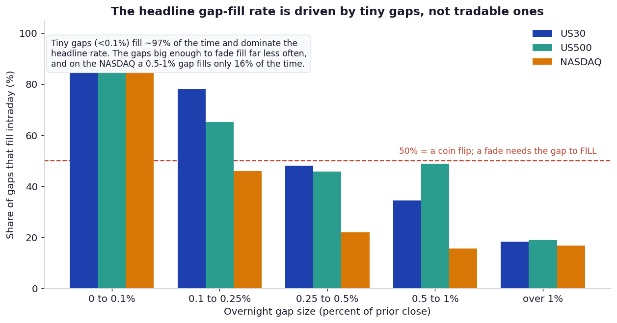
Figure 1: Gap-fill rate by gap size. Gaps under 0.1% fill about 97% of the time and make up the bulk of all gaps, which is what produces the ~90% headline. The gaps actually worth fading fill far less often: a 0.5 to 1% gap on the NASDAQ fills only 16% of the time, well below the coin-flip line a fade needs.
The mechanism is mundane. A tiny overnight gap is noise that the first few minutes of trading erase, so it "fills" almost automatically and is far too small to fade after spread. A large gap is information (an earnings reaction, a macro surprise, an overnight move abroad), and information does not politely reverse; more often it continues. The fillable gaps are not tradable and the tradable gaps do not fill.
3.3 Trading it
Sweeping the minimum gap threshold on US30, no configuration comes close to buy-and-hold:
| Min gap | Trades | Win rate | PnL after cost (pts) | Profit factor | vs buy-and-hold (+19,302) |
|---|---|---|---|---|---|
| 0.00% | 1,412 | 93.0% | +122 | 1.00 | −99% |
| 0.05% | 484 | 83.9% | +1,401 | 1.08 | −93% |
| 0.10% | 245 | 73.1% | −658 | 0.96 | Loss |
| 0.30% | 70 | 61.4% | +1,658 | 1.31 | −91% |
| 0.50% | 40 | 60.0% | +1,379 | 1.40 | −93% |
The best US30 result, +1,658 points, was chosen by picking the best threshold in-sample, which flatters it. Even so it captured under 9% of what holding the index returned. On US500 the best case captured 4%, and on the NASDAQ the best achievable result was negative.
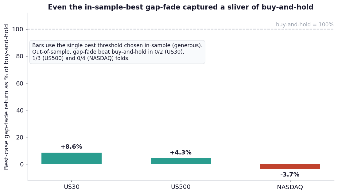
Figure 2: Best-case gap-fade return as a share of buy-and-hold (full sample, after cost). These bars use the single best threshold chosen in-sample, which is generous to the strategy, and it still captures only a sliver of buy-and-hold, turning negative on the NASDAQ. Out-of-sample it is worse: gap-fade beat buy-and-hold in 0 of 2 folds on US30, 1 of 3 on US500, and 0 of 4 on the NASDAQ.
One more tell: fade every gap with no size filter and the win rate on US500 and the NASDAQ falls below 10%, because most gaps are tiny and never travel all the way back to the prior close before the session ends. The verdict is failure on all three instruments.
4. Edges 2 and 3: IBS and RSI(2)
4.1 The claims
The IBS (Internal Bar Strength) effect, from Pagonidis (2014), measures where a day closes within its range: IBS = (close minus low) divided by (high minus low), running from 0 (close at the low) to 1 (close at the high). The verified primary finding is that days closing near their low (IBS below 0.20) are followed by an average next-day return of +0.35%, versus −0.13% after days closing near their high (IBS above 0.80). Popular reproductions of the effect report win rates around 70%. Worth noting, and rarely quoted: Pagonidis himself found the effect is essentially US-only and is hard to trade on its own net of costs, recommending it as a filter rather than a standalone signal.
Connors RSI(2), from Connors and Alvarez (2008), buys a 2-period RSI reading below an oversold threshold in an uptrend and exits on a short-term bounce. Its origin-era backtests (1995 to 2008, on the S&P 500) showed very high hit rates, often cited around 83 to 91%. It is also one of the most public examples of an edge decaying after publication; modern reproductions put the win rate closer to 58%.
4.2 The win rates
Replicated with the literature's own parameters, IBS comes in at a coin flip and RSI(2) lands in between its origin-era claim and its decayed modern figure.
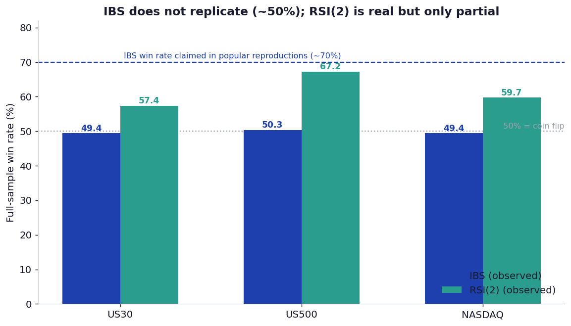
Figure 3: Observed full-sample win rates. IBS sits at 49 to 50% on all three indices, nowhere near the ~70% of its popular reproductions. RSI(2) is genuinely above a coin flip at 57 to 67%, consistent with the decayed modern figure rather than the origin-era 80s and 90s.
4.3 Profitability and out-of-sample
A win rate is not a profit. Both strategies are mildly profitable after costs on the full sample, and both underperform buy-and-hold on every instrument:
| Strategy | Win rate (US30 / US500 / NASDAQ) | Profit factor | Trades | vs buy-and-hold |
|---|---|---|---|---|
| IBS (buy below 0.20, hold 1 day) | 49.4% / 50.3% / 49.4% | 1.15 / 1.26 / 1.25 | 360 / 547 / 603 | −54% / −30% / −31% |
| RSI(2) below 5, hold 5 days | 57.4% / 67.2% / 59.7% | 1.48 / 1.64 / 1.45 | 47 / 61 / 62 | −62% / −63% / −72% |
RSI(2) shows the trap clearly. Its profit factors of 1.45 to 1.64 look respectable, but it fires only 47 to 62 times across five to eight years. It is in the market a tiny fraction of the time, so even when it is right it cannot keep up with an index that mostly trends upward.
Out-of-sample, with parameters frozen after training, the picture is decisive. The walk-forward aggregates:
| Strategy | Instrument | OOS trades | Win rate | OOS PnL (pts) | Profit factor | Beat buy-and-hold? |
|---|---|---|---|---|---|---|
| IBS | US30 | 98 | 56.1% | +4,280 | 1.17 | Yes (marginal) |
| IBS | US500 | 113 | 38.9% | −2,826 | 0.54 | No |
| IBS | NASDAQ | 157 | 49.7% | +6,043 | 1.34 | No |
| RSI(2) | US30 | 34 | 55.9% | +5,926 | 1.53 | Yes |
| RSI(2) | US500 | 21 | 57.1% | −776 | 0.53 | No |
| RSI(2) | NASDAQ | 64 | 50.0% | +936 | 1.08 | No |
Counting every fold, IBS beat buy-and-hold in only 2 of 9 out-of-sample folds, and RSI(2) in 3 of 9. The one or two wins are concentrated on US30, the cheapest-to-trade instrument, and even there they are marginal. IBS fails to replicate; RSI(2) is a partial replication of a real but weak and decaying effect that does not clear the cost of trading it on these instruments.
5. Why published edges evaporate
Nothing here implies the original studies were dishonest. It illustrates the four reasons a published edge routinely fails to reach a live account, all of which are on display above:
- Different instruments. IBS was documented on US equity ETFs and is, by the author's own finding, essentially a US phenomenon. Index CFDs are a different animal.
- Omitted costs. The mean-reversion edge per trade is small. On wide-spread instruments like US500 and the NASDAQ, the spread alone can exceed it, which is why US30, the cheapest of the three, is the only one that ever flirts with profitability.
- No out-of-sample test. Full-sample profit factors above 1 look like edges until you freeze the parameters and walk them forward, at which point most of the advantage disappears.
- Decay after publication. RSI(2) is the textbook case: a real origin-era effect that arbitrage has steadily competed away, exactly as the drop from a cited ~90% to an observed ~58% suggests.
6. What survives
Two things are worth keeping. First, gap-fill is a genuine statistical regularity, but only for small gaps, and it is better understood as a fact about intraday volatility and noise than as a directional edge. Second, RSI(2) carries a real but faint mean-reversion signal that a lower-cost venue might still use as one input among many. Neither is a standalone, tradable edge on index CFDs after the spread. The honest summary is that the venue and the cost are as decisive as the signal, and a strategy is not validated until it has been tested on the instrument and the cost structure it will actually face.
7. Limitations
Three caveats. First, the cost model is deliberately simple (one representative spread, no commission or slippage), so it is optimistic relative to live execution; this only strengthens the negative conclusion, since real costs would deepen the underperformance. Second, some out-of-sample folds contain few trades, so individual fold statistics are noisy and we lean on the aggregates and on fold-beat counts rather than any single fold. Third, the full-sample figures use the literature's fixed parameters and are descriptive replications; the out-of-sample walk-forward is the part that carries the conclusion, and we keep the two clearly separate. We did not re-test the original venues, so this is a statement about CFD-tradability, not a refutation of the original results on their own data.
8. Conclusion
We took three famous mean-reversion edges and gave each its fair test on the instruments a real trader faces. Gap-fade rests on tiny gaps that carry no tradable edge. The IBS effect's high win rate does not survive contact with a different venue. RSI(2) is a genuine but decayed signal, too sparse to beat the index it trades. After a realistic spread and an honest walk-forward, none of them outperforms simply holding the market. The lesson is not that mean reversion is fake; it is that a backtest in a paper and a position in a live account are separated by costs, venue, and out-of-sample decay, and that the only number worth trusting is the one that survives all three.
References
- Pagonidis, A. S. (2014). The IBS Effect: Mean Reversion in Equity ETFs. NAAIM white paper.
- Connors, L., & Alvarez, C. (2008). Short Term Trading Strategies That Work. TradingMarkets Publishing / Connors Research.
- Stübinger, J., & Schneider, L. (2019). Statistical arbitrage with mean-reverting overnight price gaps on high-frequency data of the S&P 500. Journal of Risk and Financial Management, 12(2), 51.
- Bailey, D. H., & López de Prado, M. (2014). The deflated Sharpe ratio: correcting for selection bias, backtest overfitting, and non-normality. Journal of Portfolio Management, 40(5), 94–107.
- López de Prado, M. (2018). Advances in Financial Machine Learning. Wiley.