How Much, Not Which Way: What 106 Public Features Actually Predict About the Dow
Abstract
We set out to forecast the direction of the Dow (US30) and, after trying every model, target, and horizon, kept landing on the same flat result: a profit factor of 1.0. Instead of re-tuning, we set the trade engine aside and ran an engine-independent battery to separate the five distinct causes of a flat equity curve. Across 438,619 out-of-sample bars and 16 walk-forward folds, our features (all public, mostly price-derived) predict 60-minute realised volatility with a rank correlation of 0.70 (36 sigma above a shuffled-label null) and predict direction no better than a coin (IC 0.009, accuracy 50.8%, 0 of 106 features surviving false-discovery control). The result holds from 60 minutes to 20 days, survives a linear and a neural alternative, and is confirmed by a label-shuffle retrain null. The conclusion was not a weak model but a wrong target: size by predicted volatility, and stop forecasting direction from price.
1. What we were actually trying to do
1.1 The goal was direction
This project started with a simple, greedy ambition: forecast which way the Dow (US30) would move next. Not how much, not when, just the sign of the next move over the coming hour. If you can call direction even slightly better than a coin, the rest of a trading system is engineering. So we spent a long time on the hard part, the forecast itself.
We built a feature set of 106 inputs (described in Section 2), trained gradient-boosted trees on the forward return, and ran the whole thing through a leak-proof, monthly-expanding walk-forward. When the 60-minute target did not work, we tried 30, 120, and 240 minutes. When intraday did not work, we tried daily and multi-day horizons. When trees did not work, we tried a linear model and a neural network. We re-labelled, re-weighted, and re-tuned.
Every road led to the same place: a profit factor of almost exactly 1.0. The equity curve neither climbed nor collapsed. It drifted, trade after trade, around break-even. For a long time we read that as an engineering failure, the wrong loss function or a stop placed a few points too tight, and kept tuning. That was the mistake, and this study is the correction.
1.2 A flat curve has five different causes
A profit factor of 1.0 is not one diagnosis, it is five, and each one calls for a completely different response:
- No information. The features genuinely cannot predict the target. Stop.
- Wrong target. The features carry real information, but about something other than what we are betting on.
- Model limitation. The information is there, but the learner cannot extract it.
- Cost-bound. A real edge exists gross, but the spread eats it.
- Regime-local. An edge lives in one regime and is averaged away by the rest.
You cannot tell these apart from a PnL curve, because all five produce the same flat line. So we put the trade engine aside and asked a narrower, more honest question: does the signal exist at all, and if it does, what is it a signal of? The rest of this paper is that diagnosis.
1.3 Why this generalises beyond one instrument
The result is not a quirk of the Dow. It restates, in measured terms, one of the oldest stylised facts in quantitative finance: returns are very close to a martingale, while their second moment, volatility, is strongly autocorrelated and forecastable (Cont, 2001). The contribution here is the discipline of the test, an engine-independent battery that separates "we found no edge" from "there is no edge to find," and reports the statistical power it had to tell the two apart.
2. The data and the features
2.1 Everything here is public, and most of it is price
One point matters before any result: nothing in this feature set is exotic or proprietary. Every input is derived from publicly available data that a retail desk can pull for free, and the large majority of the 106 features are functions of the price series itself. There is no order flow, no signed volume, no dealer-gamma positioning, no paid alternative data. The feature set is, roughly:
| Group | Share | Examples | Source |
|---|---|---|---|
| Price-derived (the bulk) | ~75% | multi-scale returns, distance from moving averages, acceleration, efficiency ratio, RSI, realised volatility and ATR, Hurst and fractal dimension, candle geometry, KMeans support/resistance levels, time-of-day encodings | the US30 price feed |
| Cross-asset | ~15% | dollar-index return, S&P 500 and NASDAQ-100 moves, US30/US500 and US30/NAS100 log spreads, relative strength, a risk-on/risk-off ratio, Brent | public price feeds |
| Macro | ~10% | yield-curve slope (10y minus 2y), 5y and 10y breakeven inflation, high-yield credit spread, changes in the 10y, initial jobless claims, unemployment | FRED (free) |
This composition is the whole point. If a rich set of public, mostly price-based features cannot find direction on one of the most liquid instruments in the world, that tells you something about where directional information is not: it is not sitting in another transform of the price path. We come back to that in Section 10.
2.2 The causal frame
Every number in this study is computed out-of-sample on a causal feature frame: the exact data the live system would have seen at decision time, with no information from the future leaking backwards. This matters because the same pipeline, in an earlier and leakier form, produced spectacular backtests, profit factors above 4, that evaporated the moment a single family of features was correctly lagged. Twelve daily-level features had been mapping the completed day's close onto every intraday bar of that same day, which is a direction oracle, not a feature. Once we applied a one-period shift, $x_t \rightarrow x_{t-1}$, to every completed-period aggregate, the apparent edge collapsed to noise. That episode is why this study exists, and why we trust its nulls: the harness was caught manufacturing a fake edge once, and we have since instrumented it to catch itself.
2.3 The walk-forward
We use a monthly-expanding walk-forward over US30 minute bars: train on all data up to the start of a calendar month, predict that month out-of-sample, then roll forward and expand the training window. This yields 16 out-of-sample folds and 438,619 out-of-sample minute bars. Normalisation statistics are fit only on each fold's training window, so the test is live-consistent.
2.4 Scale-free metrics, judged before PnL
We judge the signal with scale-free statistics rather than currency, because PnL conflates signal quality with sizing, stops, and costs. The primary metric is the Spearman rank information coefficient between the prediction and the realised forward value,
$\text{IC} = \rho_{\text{Spearman}}(\hat{y},\, y_{\text{fwd}})$,
alongside directional accuracy and the Mann–Whitney AUC of the prediction against the sign of the forward move. An IC of 0, an accuracy of 50%, and an AUC of 0.50 all mean no edge.
2.5 Reporting the power of the test
A null result is only meaningful if the test could have detected an edge. We therefore report the minimum detectable IC at 80% power, computed from the standard error of a permutation null on the de-overlapped (thinned) series,
$\text{MDE} = (z_{0.975} + z_{0.80}) \cdot \text{SE}_{\text{null}} \approx 2.80 \cdot \text{SE}_{\text{null}}$.
To keep observations independent we thin the minute series by the 60-bar horizon before computing significance, so the effective sample for the direction test is 7,310 non-overlapping observations rather than the full 438,619 bars. This keeps the error bars honest and the nulls conservative.
3. Direction does not survive the test
The deployed model is a gradient-boosted tree (LightGBM) trained on the 60-minute forward return, exactly the target the live bot bets on. Out-of-sample, across all 16 folds:
| Metric | Value | No-edge reference |
|---|---|---|
| Spearman IC (direction) | +0.0092 | 0 |
| Directional accuracy | 50.79% | 50% |
| Mann–Whitney AUC | 0.5043 | 0.50 |
| Thinned IC (95% CI) | +0.0077 [−0.0159, +0.0303] | CI contains 0 |
| Permutation p-value | 0.515 | 0.50 expected |
The confidence interval straddles zero, the permutation p-value is 0.515 (a coin flip), and the point estimate sits in the dead centre of its own null distribution. There is no directional edge here to refine, tune, or re-weight.
We also report what the test could have seen. The minimum detectable IC at 80% power is 0.033, so this experiment rules out any directional edge larger than about 0.033 but cannot rule out a vanishingly small one (a caveat we return to in Section 11). The honest statement is not "direction is provably random," it is "any directional signal in these features is smaller than the noise floor of a very large, very clean test."
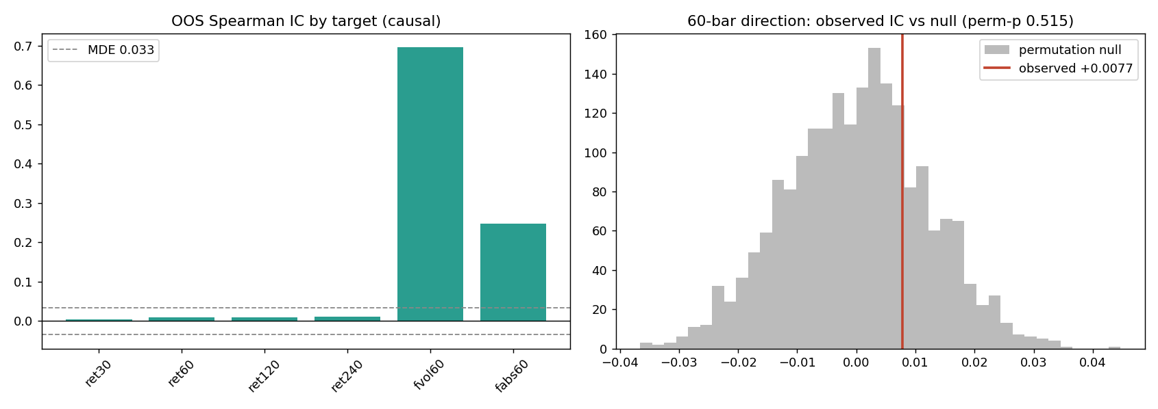
Figure 1: (Left) Out-of-sample Spearman IC by prediction target. The four directional return targets are pinned to the zero line; the volatility and absolute-move targets stand far above the dashed noise floor. (Right) The observed 60-minute direction IC (+0.0077) falls in the middle of its 2,000-draw permutation null, the definition of no signal. Raw output of the diagnosis harness.
4. It is not the model's fault
If a tree cannot find direction, perhaps a different functional form can. We ran a linear model (ridge regression) and a neural network (a small multi-layer perceptron) on the identical target and folds:
| Model | IC | Directional accuracy | AUC |
|---|---|---|---|
| LightGBM (deployed) | +0.0092 | 50.79% | 0.5043 |
| Ridge (linear) | +0.0204 | 51.29% | 0.5109 |
| MLP (neural net) | −0.0003 | 50.48% | 0.5029 |
No learner separates from chance. The linear model is nominally the best, at an AUC of 0.511, which is itself telling: if anything were really there, you would not expect a plain ridge regression to edge out a tuned tree and a neural network. This rules out the model-limitation hypothesis. The flat line is an information problem, not an architecture problem.
5. No single feature carries direction either
Maybe the model is diluting one good feature among 105 bad ones. So we bypassed the model and computed the univariate rank correlation of every individual feature against the 60-minute forward return, then applied a Benjamini–Hochberg false-discovery-rate control at $q = 0.05$ to guard against the fact that testing 106 features will throw up false positives by chance alone.
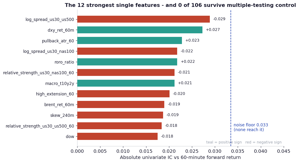
Figure 2: The twelve strongest individual features, ranked by absolute univariate IC against the 60-minute forward return. Even the best, a US30/US500 spread and a 60-minute dollar-index return, fall short of the dashed noise floor, and none survive multiple-testing control.
It is worth noting which features came closest: a cross-index spread, a dollar-index return, a risk-on/risk-off ratio, a yield-curve slope. These are the cross-asset and macro features, not the price-path features. At this effect size it is a hint rather than a finding, but it is the only direction the data points in, and we use it in Section 10.
6. Volatility, by contrast, is strongly predictable
The same features, the same model, the same folds, re-pointed at realised forward volatility instead of direction, produce a completely different picture:
| Target | Kind | IC | AUC |
|---|---|---|---|
| 60-minute return | direction | +0.0092 | 0.5043 |
| 120-minute return | direction | +0.0089 | 0.5051 |
| 240-minute return | direction | +0.0105 | 0.5049 |
| 60-minute absolute move | magnitude | +0.2470 | 0.6288 |
| 60-minute volatility | magnitude | +0.6955 | 0.8445 |
An IC of 0.70 and an AUC of 0.84 on forward volatility is not a marginal result; it is one of the strongest, cleanest signals in the whole programme. The features know almost exactly how much the market will move over the next hour. They simply have no idea which way.
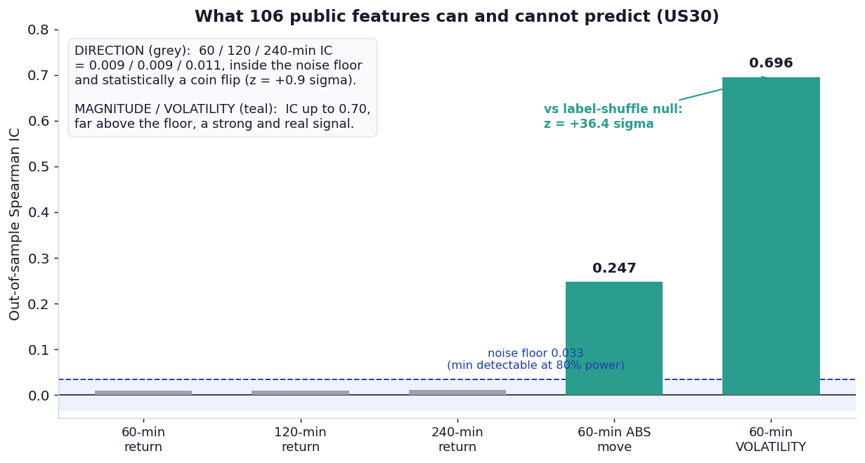
Figure 3: The whole study in one chart. Direction targets (grey) sit on the noise floor; magnitude targets (teal) tower above it. The volatility signal is 36 standard deviations above a shuffled-label null; the direction signal is 0.9, statistically invisible.
7. The harness is not lying to us
A null is only trustworthy if the test can detect a signal when one is genuinely present. To prove the harness is not simply numb, we ran a label-shuffle retrain null: permute the training labels, retrain the model from scratch, and score it against the real out-of-sample labels. If the pipeline manufactures edge from noise, the shuffled model will score above zero. We repeat this 20 times and compare the real model to the resulting null band.
| Target | Real IC | Shuffle-null IC (mean ± sd) | z-score | Verdict |
|---|---|---|---|---|
| 60-minute return (direction) | +0.0090 | +0.0016 ± 0.0081 | +0.9 | inside the null, no signal |
| 60-minute volatility | +0.6883 | −0.0033 ± 0.0190 | +36.4 | far outside, genuine signal |
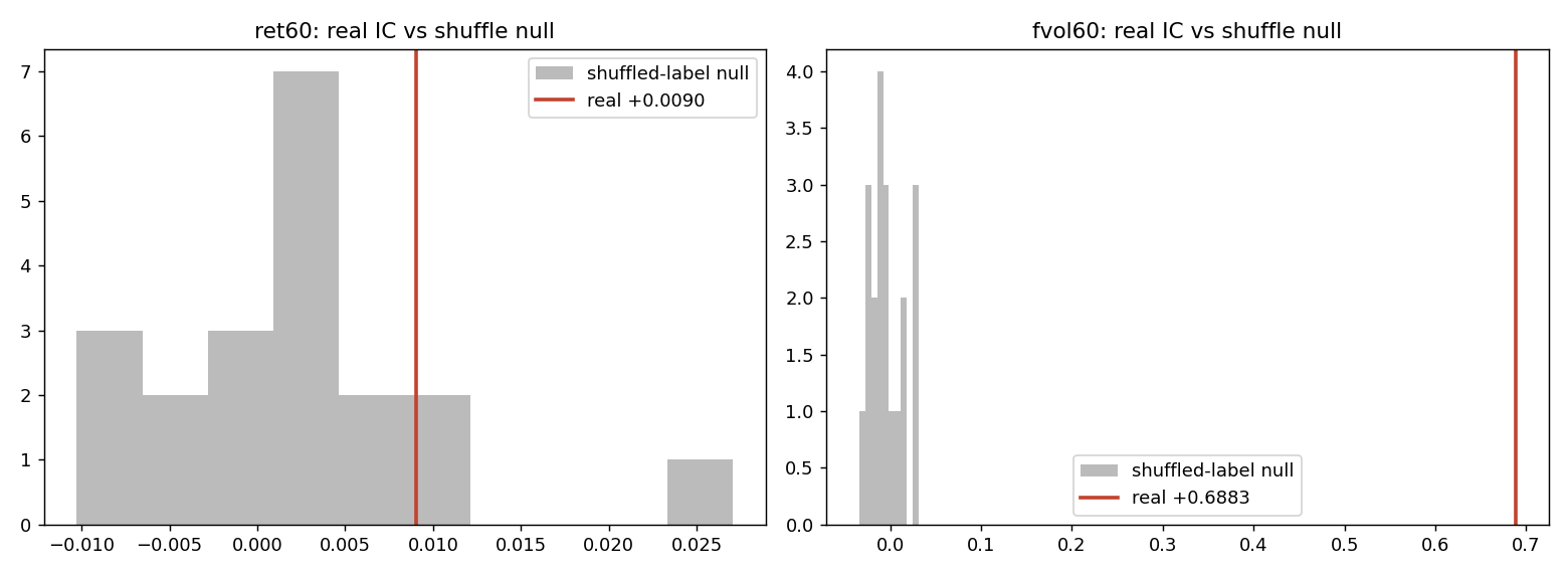
Figure 4: Label-shuffle retrain null. (Left) The real direction IC (red line) sits inside the band of models trained on shuffled labels: the direction "edge" is the same edge a model trained on scrambled targets gets by chance. (Right) The real volatility IC is nowhere near the null. This is the control that makes the direction null trustworthy: the harness clearly detects signal when there is signal to detect.
This is the single most important check in the study. The direction result is not "our model was too weak." A model trained on randomly scrambled targets does just as well. The volatility result, run through the identical machinery, lights up at 36 sigma. The instrument works; direction is simply not there.
8. It is not a horizon problem
Intraday direction being unpredictable is unsurprising. The natural rejoinder is that direction lives at a slower frequency, that daily or multi-day moves are forecastable even if hourly ones are not. So we built a separate daily-bar test: 2,602 daily observations, 49 causal daily features (momentum, moving averages, RSI, realised vol, macro, VIX, cross-asset, seasonality), 34 expanding folds, averaged over three seeds.
| Horizon | Direction IC | Directional accuracy | Clears the bar? |
|---|---|---|---|
| 1 day | −0.0099 | 50.50% | No |
| 3 days | −0.0223 | 50.65% | No |
| 5 days | −0.0109 | 51.10% | No |
| 10 days | −0.0034 | 49.21% | No |
| 20 days | +0.0103 | 51.78% | No |
Not one horizon clears its significance bar. Forward volatility, meanwhile, stays predictable at the daily scale too (IC +0.29). Direction is unpredictable from price, macro, and seasonality at both ends of the frequency spectrum, from 60 minutes to 20 days.
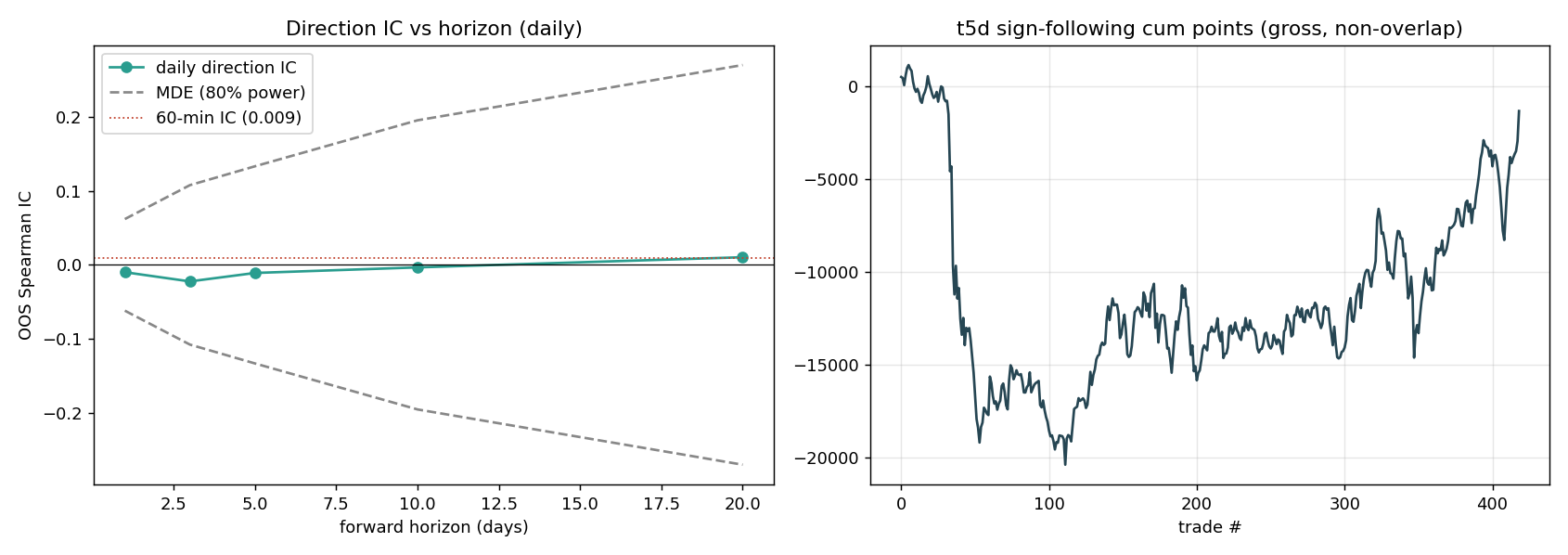
Figure 5: (Left) Daily direction IC across horizons stays pinned inside the 80%-power band; the test would see an edge if one existed, and there is none. (Right) A naive sign-follower of the 5-day signal bleeds roughly 15,000 index points over the sample before clawing some back. The point is not the exact path but that there is no monotone, exploitable drift.
9. And no regime rescues it
The last escape hatch is that an edge hides in one regime and washes out on average. We stratified the out-of-sample direction signal by volatility tercile, by trading session, and by trend sign. The best single bucket, low-volatility bars, reached a directional accuracy of 51.13%, and in the high-volatility bucket the signal actually inverts (AUC 0.493). No regime carries a standalone edge worth gating on; the spread across buckets is the random scatter you would expect from slicing noise seven ways.
Putting the economics on it: the frictionless gross edge of sign-following the deployed signal is +1.61 index points per trade, against a realistic round-trip spread of about 2.0 points. Even before asking whether that 1.61 is statistically real (it is not), it is smaller than the cost of trading it. The gross profit factor is 1.058; after spread it is 0.986. This is what the genuine absence of information looks like once you finally corner it: not a catastrophe, just a slow bleed of the spread.
10. What this changed
Of the five candidate causes, the evidence points at one: wrong target. The features are richly informative, about volatility and risk, not direction. So we changed what we do with the pipeline rather than how we tune it.
- We stopped training directional models on this feature set. A directional bot built on these features is mis-targeted by construction, and no loss function or architecture change repairs a target the data is silent on. That single conclusion retired a long backlog of "tune the model" work.
- We re-pointed the pipeline at what it predicts: volatility. An IC of 0.70 on forward vol is a bankable signal, just not a directional one. It now drives a risk throttle that scales exposure up when the next hour is predictably calm and down when it is predictably violent. We cannot bet on which way the coin lands, but we can bet on how hard, and that is enough to manage size and drawdown.
- When we look for direction again, we change the data, not the model. The features that came closest here were cross-asset and macro, not price transforms, so the next places we look are sources this study did not include, such as order flow and dealer positioning, rather than a 107th function of the same price path.
11. Limitations
A null is only as strong as the test behind it, so three caveats. First, the intraday test is well-powered only down to an IC of 0.033; a real but tiny directional edge below that floor would be invisible here, and at high frequency even a tiny edge can be tradable if costs are low enough. Second, the daily test rests on only about 2,600 observations, so a small daily-momentum effect cannot be excluded; resolving it would need a multi-instrument panel or a longer history. Third, everything here is one instrument; the result echoes a broad stylised fact, but we have not re-run the full battery on every market. None of these touches the positive result: the volatility signal is large and survives every control.
12. Conclusion
We set out to forecast the Dow's direction and spent a long time failing in a very specific way: a profit factor that sat at 1.0 no matter what we changed. The diagnosis explains the failure. These features know how much the Dow will move over the next hour and have no idea which way. That is not a modelling problem to be solved with a bigger network; it is a property of the market. Accepting it let us stop forecasting the unforecastable and put the same features to work on the part that is real: sizing and risk.
References
- Cont, R. (2001). Empirical properties of asset returns: stylized facts and statistical issues. Quantitative Finance, 1(2), 223–236.
- Benjamini, Y., & Hochberg, Y. (1995). Controlling the false discovery rate: a practical and powerful approach to multiple testing. Journal of the Royal Statistical Society: Series B, 57(1), 289–300.
- Andersen, T. G., Bollerslev, T., Diebold, F. X., & Labys, P. (2003). Modeling and forecasting realized volatility. Econometrica, 71(2), 579–625.
- López de Prado, M. (2018). Advances in Financial Machine Learning. Wiley.
- Bailey, D. H., & López de Prado, M. (2014). The deflated Sharpe ratio. Journal of Portfolio Management, 40(5), 94–107.