A Real Edge that Retail Can't Trade: A Cross-Sectional Factor Study on 1,021 US Stocks
Abstract
After a separate study found the direction of a single index to be a coin flip, we asked whether the cross-section of stocks holds the information the level does not. On 1,021 US names from 2005 to 2026, with point-in-time SEC EDGAR fundamentals and an embargoed, expanding, cost-aware walk-forward, the cross-sectional signal is genuinely real: twelve-month momentum at t = 2.76, five-day reversal at t = 2.62, and the value premium showing its two-decade drought (earnings yield t = -4.14). Yet the combined long/short book earns a net Sharpe of just 0.38, below the 0.46 deflated-Sharpe hurdle that corrects for multiple testing, and its sector-neutral refinement is worse at 0.20. The naive momentum-only sleeve lost 71% in a single month in 2009 and 96% peak-to-trough. The signal is real and, for a retail account that cannot short hundreds of names against an institutional borrow desk on survivorship-free data, untradeable. The distance between a significant t-statistic and a dollar in a real account is the subject of the paper.
1. The question behind the question
1.1 From one index to a thousand stocks
A separate study of ours ended on a deflating note: across 106 public features and every horizon we could think of, the direction of a single index is, to a good approximation, a coin flip. What that study could not answer is whether the failure was the target or the idea. Predicting the level of one index is a single bet on a single time series. Maybe the information that is missing from the level of the Dow is sitting in plain sight in the cross-section, in the gap between the stocks that are about to do well and the stocks that are about to do badly.
This is the oldest idea in quantitative equity. You do not bet on the market going up. You rank a large universe of stocks on a handful of characteristics, buy the top, short the bottom in equal dollar amounts, and collect the spread between them while staying roughly neutral to the market itself. The academic record for this is enormous and, unlike most of trading, genuinely replicated. So we built it carefully, applied the strictest validation we know, and asked a deliberately uncomfortable question: if the edge is real, can a retail account actually capture it?
But a real signal is not the same as a tradeable one. Once we build the actual long/short portfolio and charge it realistic trading costs, the profit is too small to stand apart from luck. It also needs hundreds of short positions held at the same time, it is flattered by a dataset that quietly drops the companies that went bust, and in its simplest form it lost 71% of its value in a single month during the 2009 crash. The signal is real. Capturing it from an ordinary trading account is not. The gap between those two facts is what this paper is about.
2. Data and method
2.1 Universe
We use daily closing prices for 1,021 US-listed names from 2005 to 2026 (5,397 trading days), drawn from the set of instruments available to trade rather than a clean academic database. To this we add company fundamentals scraped directly from SEC EDGAR filings: 767,220 individual XBRL facts across 1,011 companies, giving book value, earnings, revenue, profitability and share counts as reported, point-in-time. Sectors are assigned from each filer's SIC code into ten coarse buckets.
One honesty note up front, because it matters for everything that follows. The universe contains the names that survived to today. Companies that delisted, went bankrupt or were acquired on bad terms are largely absent. That omission flatters every result below, because it quietly removes some of the worst outcomes a real portfolio would have held. We did not correct for it, so read the numbers as an optimistic ceiling, not an estimate.
2.2 Factors
We rank each stock, each month, on seven price-derived factors and four fundamental ones:
- Momentum: twelve-month return skipping the most recent month (the classic form), and a three-month version.
- Reversal: the prior five-day and twenty-one-day returns, expected to predict with a negative sign (recent losers bounce).
- Risk: trailing sixty-day volatility and 120-day beta (the low-risk anomaly).
- Proximity: distance to the 52-week high.
- Value and quality: book-to-price, earnings yield, return on equity, and gross profitability, built from the EDGAR facts.
2.3 Validation
This is where most factor backtests quietly cheat, so it is where we were most careful. The portfolio is rebalanced monthly. At each rebalance a gradient-boosted model (LightGBM) is trained only on data ending a full month before the rebalance date, an embargo that prevents the label window from overlapping the training window. The training history expands over time, starting after a two-year warmup, so the model at every date sees only its own past. The model ranks the universe, we go long the top decile and short the bottom decile in equal dollar amounts, and we charge a realistic cost on every rebalance: 10 basis points per side on the names that actually turned over, plus a 2% annual borrow fee on the short book.
Finally, because we tested several factors and model variants, we do not let ourselves celebrate a positive Sharpe at face value. We compare it to a deflated-Sharpe hurdle: the Sharpe you would expect to see from the single best of N zero-edge trials, purely by chance, given the length of the sample. Only a result above that line has earned the word "edge."
3. The signal is real
Take the factors one at a time, before any portfolio is built, and measure how well each one's monthly ranking correlates with next month's returns. Two of them stand out clearly and in the textbook direction.
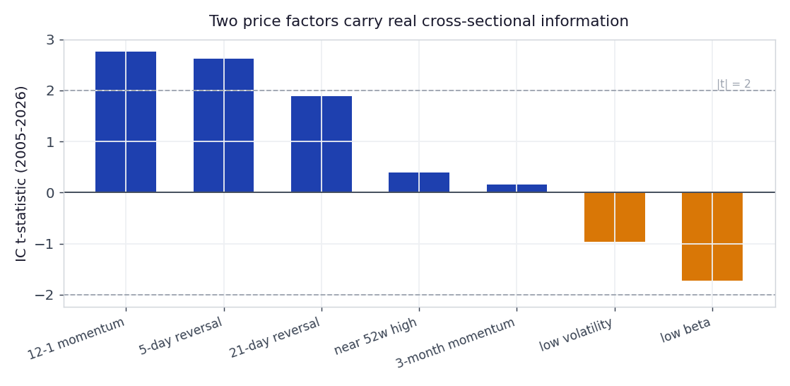
Figure 1: Information-coefficient t-statistics for the seven price factors, 2005 to 2026 (price-only specification). Twelve-month momentum (t = 2.76) and five-day reversal (t = 2.62) clear the conventional |t| = 2 line. Low-beta carries a negative sign, consistent with the low-risk anomaly, but is not significant here.
When we neutralise sectors and add the fundamentals, the picture sharpens rather than disappears. Short-term reversal strengthens to t = 3.04, momentum holds at t = 2.65, and the value factors show up with the sign that has defined the last two decades: negative. Earnings yield posts t = -4.14, meaning cheap stocks underperformed expensive ones over 2005 to 2026, the long drought of the value premium. Quality (return on equity, gross profitability) is insignificant.
| Factor | Price-only (v1) t-stat | Sector-neutral (v2) t-stat |
|---|---|---|
| 12-1 momentum | +2.76 | +2.65 |
| 5-day reversal | +2.62 | +3.04 |
| 21-day reversal | +1.89 | +2.37 |
| Earnings yield (value) | — | -4.14 |
| Book-to-price (value) | — | -2.40 |
| Return on equity (quality) | — | -1.22 |
Table 1: Cross-sectional information-coefficient t-statistics. The cross-section carries genuine, significant predictive information, which is exactly what the single-index direction study could not find. Breadth has signal where the level does not.
This is a real result and worth stating plainly. The breadth of the market is forecastable in a way the market's own direction is not. If the project had stopped here, it would read as a success.
4. The portfolio does not clear the bar
A significant information coefficient is a statement about average rank correlation. It is not a statement about money. To turn the ranking into a return we have to actually hold the long/short book, pay to trade it, and live through its path. When we do, the gross signal survives but the net result lands just short of the line.
4.1 Why a big t-statistic and a small Sharpe are the same number
This is the question the whole paper turns on, so it is worth being exact. How can momentum show a t-statistic of 2.76, which sounds emphatic, and a Sharpe ratio of barely 0.4, which is mediocre? They look like a contradiction only if you believe a t-statistic measures the size of an edge. It does not.
A t-statistic answers one question: "is the edge reliably different from zero?" It is a test of consistency. A Sharpe ratio answers a different question: "is the edge large, relative to the risk taken to capture it?" It is a measure of magnitude. A signal can be extremely reliable and still be tiny, and momentum is precisely that.
The bridge between the two is almost mechanical. A t-statistic is, near enough, the signal's information ratio multiplied by the square root of how long you measured it: $t \approx \text{IR} \times \sqrt{\text{years}}$. The momentum signal's information ratio here is about 0.6. We measured it over roughly twenty years, and the square root of twenty is about 4.5. Multiply them, 0.6 times 4.5, and you get about 2.7, which is the t-statistic. The impressive part of "2.76" is not the edge. It is the square root of two decades of patience.
And that information ratio of about 0.6 is, essentially, the gross Sharpe ratio itself (we measured 0.55). So the big t-statistic and the unimpressive Sharpe are not in tension at all. They are the same modest number, roughly 0.6, shown two ways: once on its own as the Sharpe, and once multiplied by the square root of the sample length as the t-statistic. The t-statistic only looks larger because twenty years of data inflate it. The quality of the edge was never high to begin with.
The root cause is the size of the information coefficient itself. Momentum's IC is about 0.016: a rank correlation of one and a half percent between this month's ranking and next month's returns. That is a real whisper, audible only because we hear it consistently across a thousand names and hundreds of months, but a whisper all the same. A one and a half percent rank correlation tilts the long basket only slightly above the short basket each month. Hold that thin tilt through the crash-prone volatility of the next section, then pay a spread and a borrow fee on two-thirds of the book every single month, and the thin gross edge is shaved down to a net Sharpe of 0.38, below the 0.46 bar that simply asks it to beat the luckiest of the things we tried. The high t-statistic was never a promise of profit. It was only ever a promise that this very small edge is really there.
| Specification | Gross Sharpe | Net Sharpe | Deflated hurdle | Verdict |
|---|---|---|---|---|
| v1: price-only | +0.55 | +0.38 | +0.46 | does not clear |
| v2: sector-neutral + fundamentals | +0.37 | +0.20 | +0.51 | does not clear |
Table 2: The combined machine-learning long/short book. Gross of costs the price-only version looks promising at Sharpe 0.55. Net of a realistic spread and borrow it falls to 0.38, under the 0.46 hurdle that accounts for how many factors and variants were tried.
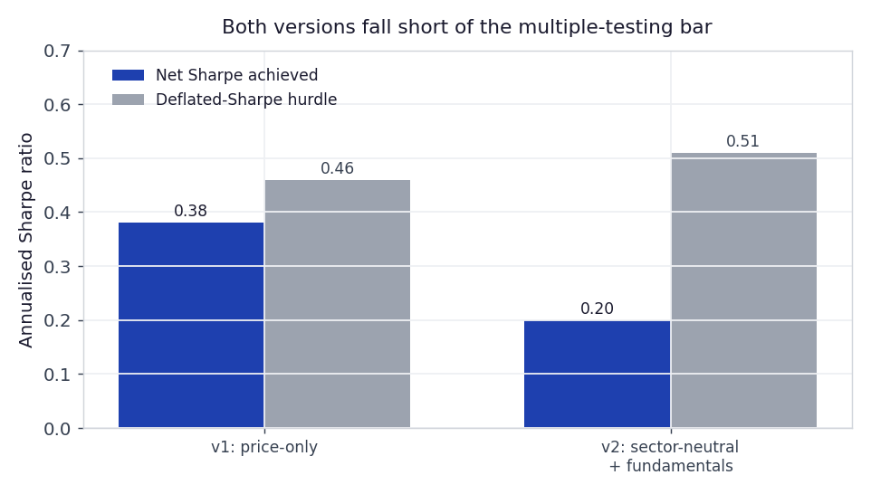
Figure 2: Net Sharpe against the deflated-Sharpe hurdle. Both specifications sit below the line they must clear to be distinguishable from the luckiest of several zero-edge trials.
Notice what the refinements did. Sector-neutralising the book and adding fundamentals, the things you are supposed to do to make a factor portfolio cleaner, roughly halved the return and pushed the result further from significance, not closer. That is itself diagnostic. It says a meaningful part of the price-only book's apparent edge was not stock-selection skill at all but unintended sector tilts and exposure to crash risk, dressed up as alpha. Strip those out and there is less left than it first appeared.
5. The path is worse than the average
Sharpe ratios are tidy. Equity curves are not, and the gap between the two is where the danger lives. The combined book did grow over nineteen years, but it did so through drawdowns that would have ended most real portfolios well before the recovery arrived.
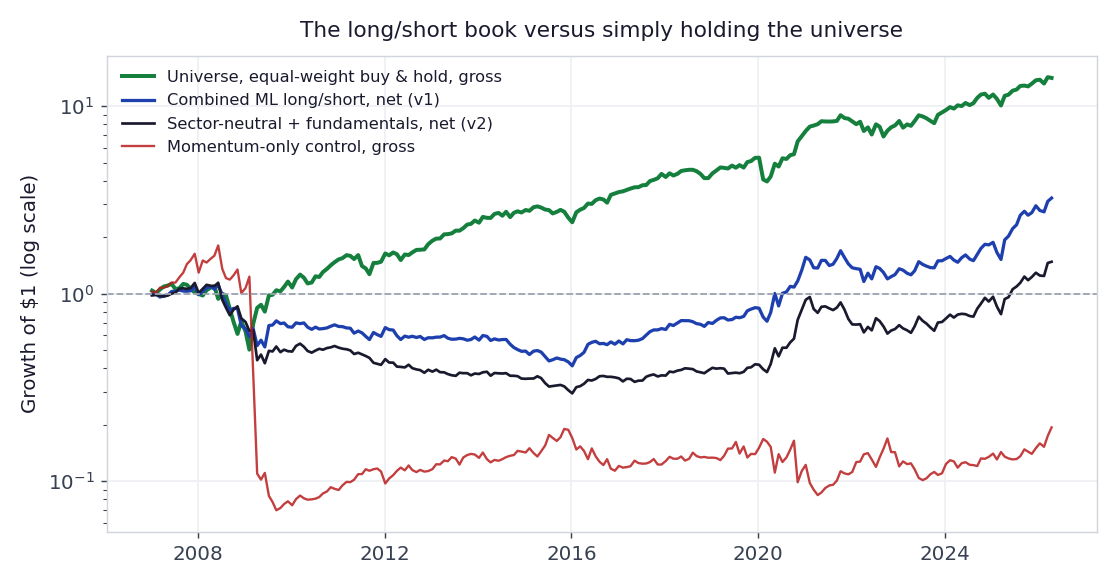
Figure 3: Growth of $1, log scale. The green line is the simplest thing a person could do: hold the whole universe, equal-weighted, rebalanced monthly. It returned about 14x. The market-neutral long/short book (blue) reached only about 3.2x, with a deeper drawdown than the market itself (63% versus 55%). Adding fundamentals (navy) made both worse. The momentum-only control (red), the single most-cited factor on its own, collapsed by 96% and never recovered. The strategy and the benchmark share the same survivorship bias, so the comparison between them is fair even though both are flattered in absolute terms.
Start with the green line, because it reframes everything beneath it. It is the least clever strategy imaginable: hold every name in the universe, in equal weight, and rebalance once a month. Over the same period it returned about fourteen times your money. The market-neutral book we worked so hard to build returned about three. Now, market-neutrality is the entire point of the design, so the book is not supposed to match the market's raw return, it deliberately strips the market out. But that is exactly what the comparison exposes: almost all of the available return was in the market itself, the part the strategy throws away, and what was left after removing it was both small and, at a 63% drawdown against the market's 55%, no gentler to hold. The book did not even earn its keep as a diversifier, because its worst moment arrived in the very crisis when an investor would have wanted protection most.
That red line is the most honest object in the study. We added a momentum-only sleeve, with no machine learning at all, to check one thing: was the problem our model, or the strategy itself? It was the strategy. In the sharp rebound of early 2009, the most beaten-down stocks suddenly doubled while the former market leaders stalled. The momentum book was, by construction, long those former leaders and short those beaten-down names, so it was caught on exactly the wrong side and lost 71% of its value in a single month. This is the well-known momentum crash, and it is not a rare accident you can diversify away. It is baked into what momentum is.
Here is the part that is easy to miss, and it is the whole point. Over the full twenty years, the momentum ranking was still right on average: its information coefficient is positive and significant. So how can something that is right on average end the period down more than 80%? Because money compounds, and compounding does not care about averages. If you lose 71% in one month, you are left with 29 cents on the dollar, and from there you have to make back +245% just to return to where you started. One or two months like that dig a hole that all the small winning months cannot climb back out of. A signal can be genuinely right in the typical month and still ruin you, because the rare disasters do not average in gently, they multiply in. This is the single most important reason a real edge and a tradeable edge are not the same thing.
6. Why retail specifically cannot trade it
Suppose you set the multiple-testing hurdle aside and decided the gross signal was worth pursuing. A large, well-financed desk might. A retail account cannot, for reasons that have nothing to do with the quality of the signal and everything to do with the venue.
- You must short hundreds of names at once. The edge lives in the bottom decile as much as the top. A market-neutral book over 1,000 stocks means roughly 100 long and 100 short positions held simultaneously, rebalanced monthly. That is an institutional prime-brokerage operation, not a retail ticket.
- Borrow is not free and not guaranteed. We charged a flat 2% annual borrow. In reality the stocks you most want to short, the worst-ranked names, are often the hardest and most expensive to borrow, exactly when you need them. Our flat fee is, again, optimistic.
- The survivorship flattery is built in. The universe already excludes the delisted and the bankrupt. A live portfolio would have held some of them on the short side (good) and some on the long side (very bad), and the historical record we tested on has quietly removed that risk.
- The multiple-testing haircut is real money, not pedantry. We tried several factors and two model designs. The deflated-Sharpe hurdle exists precisely so that the best of those tries is not mistaken for skill. Net of it, neither version clears.
Stack these together and the conclusion is not that the academic factor literature is wrong. It is right. The conclusion is that the path from a significant t-statistic to a dollar in a retail account runs through shorting infrastructure, borrow desks, clean survivorship-free data and a brutal multiple-testing correction, and that path is closed to the account most people actually have.
7. Conclusion
We set out to see whether the cross-section of stocks holds the directional information that a single index does not. It does. Momentum and short-term reversal are statistically real here, in the textbook direction, measured under an embargoed, expanding, cost-aware walk-forward that we trust. That is a genuine and slightly surprising positive result given how thoroughly direction failed at the index level.
And it changes nothing about what a retail trader should do, because the same careful framework that found the signal also shows it does not clear the multiple-testing bar net of costs, that its naive form is one of the great crash trades in market history, and that capturing even its gross version requires a venue a retail account does not have. The edge is real. The edge is not ours to trade. Holding both of those thoughts at once, rather than collapsing into either the optimism of the backtest or the cynicism of "it is all noise," is the entire discipline.
References
Bailey, D. H., and López de Prado, M. (2014). The Deflated Sharpe Ratio: Correcting for Selection Bias,
Backtest Overfitting, and Non-Normality. Journal of Portfolio Management, 40(5), 94-107.
Daniel, K., and Moskowitz, T. J. (2016). Momentum Crashes. Journal of Financial Economics, 122(2),
221-247.
Fama, E. F., and French, K. R. (1993). Common Risk Factors in the Returns on Stocks and Bonds.
Journal of Financial Economics, 33(1), 3-56.
Harvey, C. R., Liu, Y., and Zhu, H. (2016). ... and the Cross-Section of Expected Returns.
Review of Financial Studies, 29(1), 5-68.
Jegadeesh, N., and Titman, S. (1993). Returns to Buying Winners and Selling Losers: Implications for Stock
Market Efficiency. Journal of Finance, 48(1), 65-91.
López de Prado, M. (2018). Advances in Financial Machine Learning. Wiley.